Paleomagnetism:
The basic idea of paleomagnetism depends on iron bearing rock formations recording the location of the magnetic pole. By knowing where the magnetic field was then and where it is now, one can tell how much the rock formation has moved. However, if the rock had been folded or over turned, compacted, or heated can skew the results. Paleomagnetism can be a very powerful tool when trying to determine terrain transport, but is not analyzed correctly and carefully can also be very misleading.
Figure 1. (Butler 1998)
The Paleomagnetic Pole = PP, the arrows at the surface represent the dipolar magnetic field inclination with respect to PP. If a block of crust is magnetized and then displaced northward at angular distance p, the observed paleomagnetic inclination will be smaller. The latitudinal shift towards the paleomagnetic pole causes the inclination to flatten by angle F (Figure 1).
Taken from Paleomagnetism:
Magnetic Domains to Geologic Terranes: Electronic Edition
Fission Track Detrital Zircons:
Zircon grains are a detrital component of clastic sediments. The grains are accessory minerals in igneous or metamorphic rocks. Because they are very stable during erosion and transport, they are also commonly found in sediments. Trace amounts of uranium cause fission tracks to form within the crystal. The density of fission tracks is proportional to the amount of uranium in the zircon. (Geotrck 1998) Products of radiogenic decay are measured by counting the etched fission tracks under a high powered microscope (>1000x). Once a detrital zircon age distribution is measured it can be linked to an igneous or metamorphic source, providing clues on basin evolution, tectonic history, and paleogeography. Zircon age data are plotted on histograms with superimposed probability density distributions. This method does not work if the zircon is heated above its annealing temperature (240 degree C), then fission track age is reset to zero (Barnet and Spiegel 2002).
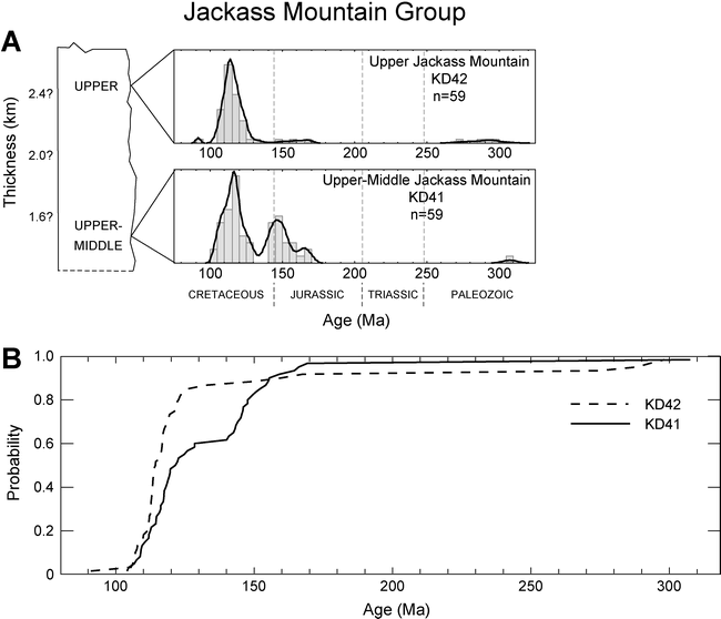
Figure 2 is an example of an age histogram and probability distribution. The bottom figure is an example of cumulative probability plots for all samples in the stratagraphic section.

Figure 2. (DeGraaff-Surpless 2003)