General Overview of the techniques
Seismic Tomography
Using the arrival times of many earthquakes (usually thousands) to stations ina particular region, it is possible to make a model of the spatial distribution of seismic velocities. It can be done using active or passive sources. The advantage of using passive sources is that the place where the energy was released is known.
A common approach to the tomography problem is to approximate the earth as a set of blocks, each of them with a specific seismic wave velocity. Given a source and a receiver, there is a ray-path that connects them. There are ray-tracing methods that allow finding an approximate trajectory of the seismic ray between the source and the receiver (Figure 8).
Figure 8 (Modified from Shearer, 1999). Ray-path along a series of 2-D blocks.
The idea is to minimize the residuals in the travel times (observed minus predicted), assuming that each block traversed by the ray has constant seismic velocity perturbation. The travel time perturbation is given by

where bij is the trajectory of the ith ray across the jth block, vj is the velocity perturbation (perturbation relative to a reference model) of the jth block and m is the number of blocks. Solving for vj involves the solution of a matrix system that usually gets so big and sometimes ill-conditioned that different numerical approaches to solve it have been proposed. If there is good ray-coverage (most of blocks in the grid are traversed by several ray-paths), we can get a spatial solution for vj with good resolution.
Seismic refraction
The main purpose of seismic refraction is to detect seismic velocity
interfaces and put some constrains in their geometry. The simplest case is to
consider a horizontal interface between two layers of constant seismic velocity.
Seismic waves are artificially generated at certain point near or on the earth’s
surface and several receivers are placed in order to get the arrivals of the
different wave fronts that are generated (figure 9).

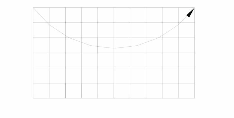
Figure 10. Wave fronts generated in a seismic refraction experiment. The angle of incidence should be the critical angle (the minimum angle for which there is no transmited wave)
A plot of first arrival time vs. traveled distance will have a break in the slope (figure 11). This represents the transition between the distances at which the first arrival is the direct wave and the distances for which the refracted wave arrives first. From the slope of the two segments it is possible to get the velocities of the top and bottom layers. The thickness of the layer can also be obtained:
![]() ,
,
where v1 and v2 are the thicknesses of the top and bottom layers respectively and ti is the intersection of the second segment of the plot arrival time vs. distance with the arrival time axis.
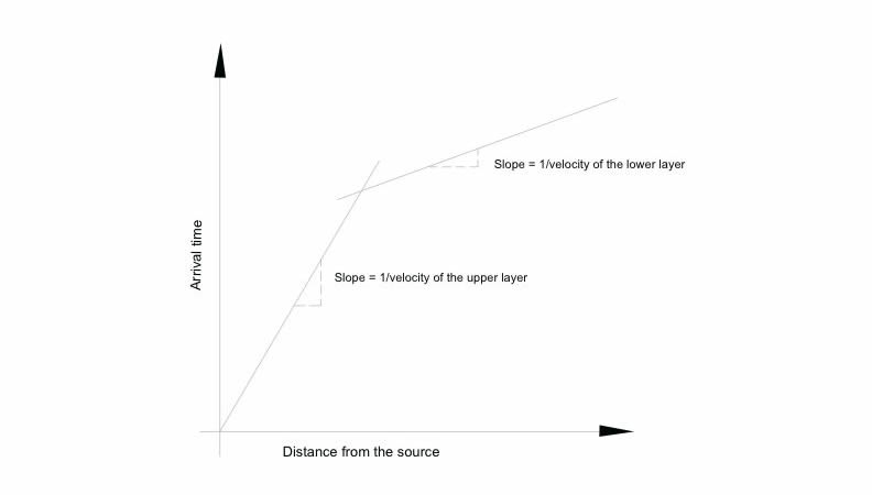
Figure 10. A break in the slope of a plot arrival time vs. distance will indicate the presence of an undergraund interface
Go to: