Cooperative Institute for Research in Environmental Sciences

---

Date: Mon, 29 Jan 2007 19:42:35 -0700 (MST)
From: Roger A Pielke Sr.
Subject: Bill Cotton class talk

Hi All, Due to a conflict Bill has, his presentation will now be on Feb 16th at the beginning of our class. Roger

---

Date: Tue, 30 Jan 2007 15:02:20 -0700 (MST)
From: Roger A Pielke Sr
Subject: simple climate models

Hi All, With the permission of Dr. Zong-Liang Yang of the University of Texas in Austin I am sharing the access information for several useful models which could help us appreciate the complexity of the climate system, even with
"simple" models. The models can be accessed at

http://www.geo.utexas.edu/courses/387h/climate_models.htm

Roger

---

Date: Sun, 4 Feb 2007 09:05:57 -0700 (MST)
From: Roger A Pielke Sr.
Subject: Class Feb 9

Hi All, We had an excellent class discussion on Friday, and I would like to continue on Friday. We will discuss the science in the newly released IPCC Statement of Policymakers

http://www.ipcc.ch/ (download pdf from here)

I also will be discussing model types and will refer to the following material I would like you to read:

1. Pielke Sr., R.A., 2002: Overlooked issues in the U.S. National Climate and IPCC assessments. Climatic Change, 52, 1-11. http://www.climatesci.org/publications/pdf/R-225.pdf

2. MacCracken, M., 2002: Do the uncertainty ranges in the IPCC and U.S. National Assessments account adequately for possibly overlooked climatic influences. Climatic Change, 52, 13-23.
http://www.climatesci.org/publications/pdf/maccracken2002.pdf

In addition, I will be showing the slides from the talk

Pielke, R.A., Sr., 2003: The Limitations of Models and Observations. COMET Symposium on Planetary Boundary Layer Processes, Boulder, Colorado, September 12, 2003. http://www.climatesci.org/presentations/PPT-3.pdf

For our Feb 16 class, after Bill Cotton's talk), we will introduce another climate forcing; the biogeochemical forcing of CO2. Papers to read include (and I am asking Dallas to add the pdf links for the ones listed below)

1. Cox, P. M., R. A. Betts, C. D. Jones, S. A. Spall, and I. J. Totterdell. 2000. Acceleration of global warming due to carbon-cycle feedbacks in a coupled climate model. Nature 408:184-187.

2. Friedlingstein P., L. Bopp, P. Ciais, J.-L Dufresne, L. Fairhead, H. LeTreut, P. Monfray, and J. Orr. 2001. Positive feedback between future climate change and the carbon cycle. Geophysical Research Letters 28:1543-1546.

3. http://www.terradaily.com/2006/061212004701.x492i9mu.html  See discussion on this news release at
http://www.climatesci.org/2006/12/12/additional-evidence-of-the-complex-role-of-vegetation-in-climate-change/]

4. Pielke Sr., R.A., 2001: Carbon sequestration . The need for an integrated climate system approach. Bull. Amer. Meteor. Soc., 82, 2021. Bull. Amer. Meteor. Soc., 82, 2021. http://www.climatesci.org/publications/pdf/R-248.pdf

5. Eastman, J.L., M.B. Coughenour, and R.A. Pielke, 2001: The effects of CO2 and landscape change using a coupled plant and meteorological model. Global Change Biology, 7, 797-815. http://www.climatesci.org/publications/pdf/R-229.pdf

6. Pielke Sr., R.A., G. Marland, R.A. Betts, T.N. Chase, J.L. Eastman, J.O. Niles, D. Niyogi, and S. Running, 2002: The influence of land-use change and landscape dynamics on the climate system- relevance to climate change policy beyond the radiative effect of greenhouse gases. Phil. Trans. A. Special Theme Issue, 360, 1705-1719.
http://www.climatesci.org/publications/pdf/R-258.pdf

Roger

---

Date: Sun, 4 Feb 2007 12:09:39 -0700 (MST)
From: Roger A Pielke Sr.
Subject: Visit

We will be fortunate to have an outstanding visiting speaker in our class this Friday (Feb 9), so the earlier schedule for what we would be talking on is deferred until the 16th and 23rd. I have asked her (Bridget Scanlon) to present both of the very interesting and important topics that are given below. I am also inviting others in CIRES and ATOC to attend, including members of my research group (who are also included on this e-mail). See all of you Friday! Roger

Bridget Scanlon, Birdsall-Dreiss Distinguished Lecturer for 2007

Bridget Scanlon of the University of Texas at Austin, has been selected as the 2007 Birdsall-Dreiss Distinguished Lecturer, sponsored by the GSA Hydrogeology Division. At the request of institutions, she will present one of two lectures for audiences interested in broad aspects of water resources.

Bridget Scanlon received a B.S. in Geology at Trinity College, Dublin (Ireland), an M.S. at the University of Alabama, and a Ph.D. from the University of Kentucky (Lexington).  She is currently a Senior Research Scientist at the Bureau of Economic Geology, the Jackson School of Geosciences. The primary objective of her research group is to assess sustainability issues with respect to water resources, within the context of climate variability and land-use change. Studies integrate physical, chemical, and isotopic analyses and numerical modeling. Much of her research focuses on groundwater recharge in semiarid regions in natural and cultivated ecosystems. Bridget Scanlon has taught Vadose Zone Hydrology at the Dept. of Geological Sciences and Civil Engineering at UT. She participated in focus groups on global recharge issues within the IAEA. She served on NAS committees on radioactive waste disposal and is currently serving on the Integrated Observations on Hydrologic Sciences committee.

To request a visit to your institution contact Bridget Scanlon, Bureau of Economic Geology, Jackson School of Geosciences, Univ. of Texas at Austin, J.J. Pickle Research Campus, Bldg, 130, 10100 Burnet Rd., Austin, TX 78758-4445, 512 471 8241, bridget.scanlon@beg.utexas.edu.  The deadline for requests is December 15, 2006. The Division will pay transportation expenses and the host institution will provide local accommodations.

Talk Topics

Implications of Climate Variability for Groundwater Resources and Waste Disposal in Semiarid Regions – A Look at Ecological Controls from Annual to Millennial Timescales

Understanding impacts of climate variability on groundwater recharge is essential for management of water resources and waste disposal. Water scarcity is a critical issue in semiarid regions and potential contaminant transport by recharge to groundwater is also important because of waste disposal. A key question is how do climate variability and related vegetation dynamics impact groundwater recharge.

This talk will explore the role of vegetation dynamics in regulating the impact of climate variability on groundwater recharge. Results from a unique field data set from weighing lysimeters (large, soil-filled concrete containers) beneath nonvegetated and vegetated systems in the Mojave Desert, Nevada unequivocally show that vegetation dynamics controls the impact of elevated winter precipitation related to El Nino Southern Oscillation (ENSO) on groundwater recharge. The lysimeter data indicate that rapid increases in vegetation productivity in response to 2.5 times normal winter precipitation reduced soil water storage to half of that in the nonvegetated lysimeter; thereby precluding deep drainage below the root zone that would otherwise result in groundwater recharge. Satellite vegetation data provided regionalization of the “point scale” lysimeter results. Unsaturated zone chloride and pressure data at sites across the southwestern U.S. indicate that similar feedbacks have minimized inter-stream basin-floor recharge since the last glacial period, 10,000–15,000 years ago. Strong correlations between satellite vegetation productivity and interannual precipitation variability related to ENSO in deserts in Australia, South America, and Africa indicate that the processes described in the southwestern U.S. may apply to deserts globally. The two-way coupling between the water cycle and vegetation dynamics is critical in controlling how climate variability influences water resources, with important implications for waste disposal in semi-arid regions.

References

Scanlon, B. R., D. G. Levitt, K. E. Keese, R. C. Reedy, and M. J. Sully. 2005. Ecological controls on water-cycle response to climate variability in deserts. Proceedings of the National Academy of Sciences of the United States of America 102:6033-6038.
Scanlon, B. R., K. Keese, R. C. Reedy, J. Simunek, and B. J. Andraski. 2003. Variations in flow and transport in thick desert vadose zones in response to paleoclimatic forcing (0-90 kyr): field measurements, modeling, and uncertainties. Water Resources Research 39:1179; doi:1110.1029/2002WR001604.

Impacts of Changing Land Use on Subsurface Water Resources in Semiarid Regions

The most widespread changes in land use have occurred because of agricultural expansion. In the past 300 years, cultivated cropland and pastureland have increased globally by 560% and 660%, respectively. Irrigated agriculture has expanded by 580% since 1900 and is projected to increase by 20% by 2030 in developing countries Agricultural food production accounts for ~85% of global fresh water consumption, led by irrigated agriculture. What impacts have these land-use changes had on water resources?

Measurements of pressure head, soil pore water chemistry, groundwater levels, and groundwater quality provide an archive of system response to past land-use changes. The presentation will focus on the Texas Southern High Plains, which is one of the largest agricultural areas in the United States. Cultivation of natural grasslands has changed the system from discharging through evapotranspiration since Pleistocene times (~10,000 to 15,000 yr) to recharging during the past 50 to 100 yr. Recharge under rain-fed agriculture is shown by large groundwater-level rises (average 7 m over 3,400 km2 area of rain-fed agriculture) during the last few decades, resulting in a median recharge rate of 21 mm/yr (5% of precipitation). Changes from discharge to recharge conditions reflect long fallow periods (~7 months/yr) associated with cultivation. Recharge under irrigated agriculture is shown by downward hydraulic head gradients. Large groundwater-level declines (as much as 75 m) under irrigated areas indicate that irrigated agriculture is not sustainable. Results from land-use changes in this region will be compared with those from other regions globally. Although past land-use changes had unintended impacts on the water cycle, a comprehensive understanding of these impacts could be used to alter land-use practices for better management of water resources.

References

Scanlon, B. R., I. D. Jolly, M. Sophocleous, and L. Zhang. in press. Global impacts of agricultural land-use changes on water resources: quantity versus quality. Water Resour. Res.
Scanlon, B. R., R. C. Reedy, D. A. Stonestrom, D. E. Prudic, and K. F. Dennehy. 2005. Impact of land use and land cover change on groundwater recharge and quality in the southwestern USA. Global Change Biology 11:1577-1593.

---

Date: Mon, 05 Feb 2007 13:19:49 -0700
From: Carl Drews
Subject: Comments on Dr. Pielke's hurricane articles

Dr. Pielke handed out a set of articles on hurricanes and climate.  I made some comments and passed them along to Josh McGrath. I found it useful to include some figures with my comments.  These figures are in the attached document.  PDF

---

Date: Thu, 8 Feb 2007 16:02:02 -0700 (MST)
From: Roger A Pielke Sr
Subject: webcast of Hearing on the IPCC report

Hi All, Thanks for to Marcia, the webcast of today's Hearing can be heard at
http://science.house.gov/publications/hearings_markups_details.aspx?NewsID=1264

The State of Climate Change Science 2007: The Findings of the Fourth Assessment Report by the Intergovernmental
Panel on Climate Change (IPCC), Working Group I Report

Roger

---

Date: Mon, 12 Feb 2007 10:13:33 -0700 (MST)
From: Roger A Pielke Sr.
Subject: Friday class

Hi All, Friday, Bill Cotton will present a talk in the first part of class. We will cover the papers listed in the course information listed on Tue 30 Jan 2007 15:02:20 -0700 (MST) and Sun, 4 Feb 2007 09:05:57 -0700 (MST) on
the course website (and earlier dates where we have not yet covered the papers completely)
http://cires.colorado.edu/science/groups/pielke/classes/atoc7500/

On the list of papers under the different climate metrics listed at the bottom of the class website, please send Dallas urls for papers to add to the list (which she can do when she returns in two weeks). Roger

---

Date: Mon, 12 Feb 2007 15:52:06 -0700 (MST)
From: Roger A Pielke Sr.
Subject: Re: Lecture a week from tomorrow

Hi All, The talks that are mentioned below would be of interest. Please attend if you can and report back to class on what you learned. I will be giving a talk to his class on the 20th, and he okayed that you could attend any of
the other talks. [I suggest asking him for a schedule]. Roger

---

Date: Tue, 13 Feb 2007 13:17:33 -0700 (MST)
From: Roger A Pielke Sr.
Subject: Friday's talk

Hi All, Bill Cotton's talk on Friday is titled "Aerosol Influences on Clouds and Precipitation"

He may also present material from another talk on his view of climate change.

Please invite your colleagues to attend also. Roger

---

Date: Thu, 15 Feb 2007 08:00:14 -0700 (MST)
From: Roger A Pielke Sr.
Subject: Fw: CSD seminar, Wednesday Feb 21, Susan Solomon (fwd)

Hi All, This seminar would be of interest and relevance to our class if you can attend. Roger

From: Karen Rosenlof
Sent: Wednesday, February 14, 2007 4:46 PM
To: seminars.csd@noaa.gov
Subject: CSD seminar, Wednesday Feb 21, Susan Solomon

NOAA CHEMICAL SCIENCES DIVISION SEMINAR NOTICE
Earth System Research Laboratory (ESRL) Chemical Sciences Division
(CSD), formerly programs of the Aeronomy and Environmental Technology Laboratories

SPEAKER:Susan Solomon, NOAA ESRL CSD
TIME: WEDNESDAY, February 21, 2007, 3:30 pm
PLACE: DSRC (NOAA Building) Room GC-402 (Skaggs Multipurpose room), 325 Broadway, Boulder
DIRECTIONS: See http://esrl.noaa.gov/csd/seminars/
NOTE:  This is not in the normal CSD seminar room.

TITLE: IPCC (2007) Climate Change: The Physical Science Basis

ABSTRACT: This talk will present a comprehensive overview of the key scientific findings of the 2007 report of Working Group 1 of the Intergovernmental Panel on Climate Change.

***NOTE***  All visitors, including pedestrians and bike riders, must check in and receive a temporary badge at the Dept. of Commerce entrance on Broadway. Please contact Karen Rosenlof at 303-497-7761 with any questions.  For entry onto the NOAA site, use either Karen Rosenlof (X7761) or Brenda Irish (X3429) as your contact for security.
For more information see http://www.esrl.noaa.gov/csd/seminars/

Karen Rosenlof
NOAA ESRL Chemical Sciences Division
Mail Stop R/CSD-6
325 Broadway
Boulder, CO 80305
office: 2A-135, DSRC

---

Date: Thu, 15 Feb 2007 08:46:17 -0700 (MST)
From: Roger A Pielke Sr.
Subject: aerosol climate forcings

Hi All

In order to properly discuss aerosol climate forcings, we need to understand the jargon words that are used to define the different types of forcings. The 2005 NRC report can be used to introduce the focrings:

I. Direct Effect of Aerososl (text starting on page 34 of
http://books.nap.edu/openbook.php?chapselect=yo&page=34&record_id=11175&Jump+to+Specified+Page.x=14&Jump+to+Specified+Page.y=9)

i) those that are dominated by scattering

ii) those that are domionated by absorption

II. Indirect Effect of Aerosols

i)  First Indirect Effect

ii) Second Indirect Effect

iii) Semidirect Effect

iv) Glaciation effect

v) Thermodynamic Effect

vi) Surface energy Budget Effect

[these forcings are discussed also in the 2005 NRC report starting on page 39
http://books.nap.edu/openbook.php?chapselect=yo&page=39&record_id=11175&Jump+to+Specified+Page.x=11&Jump+to+Specified+Page.y=14]

vii) atmospheric deposition

a) black carbon (see page 38 in the 2005 NRC report
http://books.nap.edu/openbook.php?chapselect=yo&page=38&record_id=11175&Jump+to+Specified+Page.x=10&Jump+to+Specified+Page.y=14

b) nitrogen deposition (see
http://www.climatesci.org/2005/10/10/is-nitrogen-deposition-a-first-order-climate-forcing/)

viii) Others?

As an assignment, please search the literature on google or other search engine and find the more recent review paper and other papers on each of the forcings. We will discuss in class, including how well the new IPCC Statement for Policymakers included these forcings. Please e-mail the class papers that you find. We will discuss the papers that are found.

Roger

---

Date: Thu, 15 Feb 2007 09:52:12 -0700 (MST)
From: Roger A Pielke Sr.
Subject: Climate Model Prediction skill

Hi All, Please add this paper to the set we will discuss this semester.

Jiouni R, 2007: "How reliable are climate models?" Tellus A 59 (1), 2.29.  doi:10.1111/j.1600-0870.2006.00211.x

Roger

---

Date: Thu, 15 Feb 2007 14:15:20 -0700 (MST)
From: Roger A Pielke Sr.
Subject: Guest Speaker - Dr. De-Zheng Sun

Hi All, We are fortunate to have Dr. Sun agree to present a one hour talk to our class on March 2 at 8am. Please also let your colleagues know of this informative presentation.

"Validating and Understanding Feedbacks in Climate Models"

Roger

---

Date: Thu, 15 Feb 2007 14:32:26 -0700
From: Laure Montandon

Subject: aerosol indirect effects - recent work

Hi all, Here is the most recent paper (2005, see attachment) I could find on the effects of aviation on radiative forcing:

Do aircraft black carbon emissions affect cirrus clouds on the global scale?
Hendricks J, Karcher B, Lohmann U, Ponater M
GEOPHYSICAL RESEARCH LETTERS 32 (12): Art. No. L12814 JUN 24 2005

Abstract
Potential cirrus modifications caused by aircraft-produced black carbon (BC) particles via heterogeneous ice nucleation were studied with a general circulation model. Since the role of BC in cirrus cloud formation is currently not well known, hypothetical scenarios based on various assumptions on the ice nucleation efficiency of background and aircraft-induced BC particles were considered. Using these scenarios, the sensitivity of ice cloud microphysics to aviation-induced BC perturbations is studied. The model results suggest that cloud modifications induced by aircraft BC particles could change the ice crystal number concentration at northern midlatitudes significantly (10--40% changes of annual mean zonal averages at main flight altitudes), provided that such BC particles serve as efficient ice
nuclei. The sign of the effect depends on the specific assumptions on aerosol-induced ice nucleation. These results demonstrate that, based on the current knowledge, significant cirrus modifications by BC from aircraft cannot be excluded.

I also found a 2005 review paper on indirect aerosols effects that I is the most recent review on the topic (download it from
http://www.atmos-chem-phys.org/5/715/2005/acp-5-715-2005.pdf):

Global indirect aerosol effects: a review U. Lohmann1 and J. Feichter2
1ETH Institute of Atmospheric and Climate Science, Schafmattstr. 30, CH-8093 Zurich, Switzerland
2Max Planck Institute for Meteorology, Bundesstr. 53, D-20146 Hamburg, Germany
Received: 7 October 2004 -- Published in Atmos. Chem. Phys. Discuss.: 17 November 2004
Revised: 28 January 2005 -- Accepted: 18 February 2005 -- Published: 3 March 2005

Laure

---

Date: Thu, 15 Feb 2007 14:46:23 -0700
From: Carl Drews
Subject: Greenland ice sheet

The Greenland Ice Sheet

I was not able to attend Koni Steffen's talk this morning, but I did poke around a bit on his website: http://cires.colorado.edu/steffen/

He appears to be concentrating on areas of _surface_ melt.  The total area of surface melt is increasing, as this nifty 3-D diagram shows: http://cires.colorado.edu/steffen/greenland/melt2005/melt2005PS2.5inch.jpg

That's impressive!  And it's obvious that some kind of unusual warming is taking place in Greenland, because areas are now melting that never melted before. Unfortunately, surface melt addresses the total mass balance only indirectly. Greenland might be re-gaining that melt due to increased precipitation.

Here is some information on the Greenland ice sheet: http://en.wikipedia.org/wiki/Greenland_ice_sheet

The total volume of the ice sheet is estimated at 2.85e6 km3.  That's equivalent to 7.2 meters of sea level rise.  That would be a problem.

The rate of melting appears to be accelerating; during 1996 96 km3 was lost, in 2005 220 km3 was lost, and in 2006 the net loss of mass was estimated at 239 km3 annually.

Now, 239 km3 is a lot of ice if it's all in your driveway, but when considered against the total volume of the ice sheet it's only 0.0084 percent change.  You could not see that change on a graph.  At that rate it would take over 100 years just to accumulate a full 1% change in volume (as long as the rate of loss stays constant).  Isn't it amazing that satellites can measure the Greenland ice volume so accurately?  If I were a policy maker I would be tempted to say, "Wake me up when the mass loss goes over 1,000 km3 per year.  Until then, don't bother me."

If the increase is _exponentially_ increasing then the picture changes drastically.  I'll admit that this is a huge extrapolation, but suppose we take the three data points as representative of a exponentially increasing curve. After some algebra, we have

Ice loss per year = 10 ^ (0.04 * year - 77.86)

At that rate, the entire Greenland ice sheet is melted away by the year 2082.  I guess the point here is that exponential processes can really get out of hand in a couple of human generations.  Does anyone know if exponential ice loss is at all realistic?

If we assume a linear rate of increase in melting, then the Greenland ice sheet lasts until the year 2621.  The annual loss rate is up to 9,033.5 km3 by then.

Linear ice loss per year = 14.3 * year - 28,446.8

Carl

---

Date: Thu, 15 Feb 2007 16:41:02 -0700
From: Marcia Wyatt
Subject: papers on aerosols

Hi All, I have a few to offer. One is the one I sent early in the semester, the one showing effects on Arctic clouds by Lubin et al.

Another by Ackerman et al. discusses soot's effect on tropical clouds.

The last is on organic aerosols in the troposphere and their absence in models by Heald et al.

They are all attached. See you tomorrow. Marcia

---

Date: Fri, 16 Feb 2007 06:57:37 -0700
From: Marcia Wyatt
Subject: Re: aerosol climate forcings

Hi all, I sent some articles yesterday. In fact I did it twice (my incompetence showing), but this morning I had a "mail delivery failure" in my box. If you didn't get the aerosol articles, please write me and I'll send.

I have an article I'd like to share. It discusses CO2 and heat uptake by the oceans. This article (attached) discusses the placement of the ACC in models. The authors of this article note that if it is positioned more poleward, to reflect its accurate location, uptake of both parameters is increased. Models do not have the ACC accurately placed.

"The Southern Hemisphere Westerlies in a Warming World: Propping Open the Door to the Deep Ocean" by Russell et al.

Marcia

---

Date: Fri, 16 Feb 2007 18:27:12 -0700 (MST)
From: Roger A Pielke Sr.
Subject: CCNet: ANTARCTIC TEMPERATURES DISAGREE WITH CLIMATE MODEL
    PREDICTIONS (fwd)

Hi All, The news article below is interesting in light of the upcoming February 19 INSTAAR talk by Peter Barrett "Antarctic climate history - deep past and near future" (Laure - thank you for letting us know about the talk!).

Clearly, there are different views on this subject. Roger

P.S. If you would like to subscribe (its free) to CCNet, please contact them to join. There are usually items of relevance to our class. For climate websites, I recommend Climate Audit and Real Climate as two different viewpoints with both well respected.
++++++++++++++++++++++++

CCNet 36/07 - 16 February 2007 -- Audiatur et altera pars
ANTARCTIC TEMPERATURES DISAGREE WITH CLIMATE MODEL PREDICTIONS
--------------------------------------------------------------


A new report on climate over the world's southernmost continent shows that temperatures during the late 20th century did not climb as had been predicted by many global climate models. It follows a similar finding from last summer by the same research group that showed no increase in precipitation over Antarctica in the last 50 years. Most models predict that both precipitation and temperature will increase over Antarctica with a warming of the planet.
--Physorg.com, 15 February 2007


It's hard to see a global warming signal from the mainland of Antarctica right now. The best we can say right now is that the climate models are somewhat inconsistent with the evidence that we have for the last 50 years from continental Antarctica. We're looking for a small signal that represents the impact of human activity and it is hard to find it at the moment.
    --David Bromwich, Byrd Polar Research Center, 15 February 2007


We didn't know as much about the Antarctic ice sheet as we thought we did.
--Helen Fricker, Scripps Institution of Oceanography, 15 February 2007


Not since The Hitchhiker's Guide to the Galaxy has an author appeared to have so much fun wiping out humanity. This thinking leads in only one direction: the total state, to protect us from ever-more-dangerous hypothetical evildoers and technologies.... Governments killed at least 170 million of their own people in the twentieth century, and countless more through war. That was a catastrophe for humanity. It will be again if we follow the path Richard Posner has laid out for us.
--J.H. Huebert, 5 February 2007


(1) ANTARCTIC TEMPERATURES DISAGREE WITH CLIMATE MODEL PREDICTIONS
Physorg.com, 15 February 2007

(2) PREDICTING FATE OF GLACIERS PROVES SLIPPERY TASK
Richard A. Kerr, ScienceNOW Daily News, 15 February 2007

===============
(1) ANTARCTIC TEMPERATURES DISAGREE WITH CLIMATE MODEL PREDICTIONS

Physorg.com, 15 February 2007
http://www.physorg.com/news90782778.html

A new report on climate over the world's southernmost continent shows that temperatures during the late 20th century did not climb as had been predicted by many global climate models.

This comes soon after the latest report by the Intergovernmental Panel on Climate Change that strongly supports the conclusion that the Earth's climate as a whole is warming, largely due to human activity.

It also follows a similar finding from last summer by the same research group that showed no increase in precipitation over Antarctica in the last 50 years. Most models predict that both precipitation and temperature will increase over Antarctica with a warming of the planet.

David Bromwich, professor of geography and researcher with the Byrd Polar Research Center at Ohio State University, reported on this work at the annual meeting of the American Association for the Advancement of Science at San Francisco.

"It's hard to see a global warming signal from the mainland of Antarctica right now," he said. "Part of the reason is that there is a lot of variability there. It's very hard in these polar latitudes to demonstrate a global warming signal. This is in marked contrast to the northern tip of the Antarctic Peninsula that is one of the most rapidly warming parts of the Earth."

Bromwich says that the problem rises from several complications. The continent is vast, as large as the United States and Mexico combined. Only a small amount of detailed data is available - there are perhaps only 100 weather stations on that continent compared to the thousands spread across the U.S. and Europe. And the records that we have only date back a half-century.

"The best we can say right now is that the climate models are somewhat inconsistent with the evidence that we have for the last 50 years from continental Antarctica.

"We're looking for a small signal that represents the impact of human activity and it is hard to find it at the moment," he said.

Last year, Bromwich's research group reported in the journal Science that Antarctic snowfall hadn't increased in the last 50 years. "What we see now is that the temperature regime is broadly similar to what we saw before with snowfall. In the last decade or so, both have gone down," he said.

In addition to the new temperature records and earlier precipitation records, Bromwich's team also looked at the behavior of the circumpolar westerlies, the broad system of winds that surround the Antarctic continent.

"The westerlies have intensified over the last four decades of so, increasing in strength by as much as perhaps 10 to 20 percent," he said. "This is a huge amount of ocean north of Antarctica and we're only now understanding just how important the winds are for things like mixing in the Southern Ocean." The ocean mixing both dissipates heat and absorbs carbon dioxide, one of the key greenhouse gases linked to global warming.

Some researchers are suggesting that the strengthening of the westerlies may be playing a role in the collapse of ice shelves along the Antarctic Peninsula.

"The peninsula is the most northern point of Antarctica and it sticks out into the westerlies," Bromwich says. "If there is an increase in the westerly winds, it will have a warming impact on that part of the continent, thus helping to break up the ice shelves, he said.

"Farther south, the impact would be modest, or even non-existent."

Bromwich said that the increase in the ozone hole above the central Antarctic continent may also be affecting temperatures on the mainland. "If you have less ozone, there's less absorption of the ultraviolet light and the stratosphere doesn't warm as much."

That would mean that winter-like conditions would remain later in the spring than normal, lowering temperatures.
"In some sense, we might have competing effects going on in Antarctica where there is low-level CO2 warming but that may be swamped by the effects of ozone depletion," he said. "The year 2006 was the all-time maximum for ozone depletion over the Antarctic."

Bromwich said the disagreement between climate model predictions and the snowfall and temperature records doesn't necessarily mean that the models are wrong.

"It isn't surprising that these models are not doing as well in these remote parts of the world. These are global models and shouldn't be expected to be equally exact for all locations," he said.

Source: Ohio State University

Copyright 2007, Physorg.com

===========
(2) PREDICTING FATE OF GLACIERS PROVES SLIPPERY TASK

ScienceNOW Daily News, 15 February 2007
http://sciencenow.sciencemag.org/cgi/content/full/2007/215/2

By Richard A. Kerr

Earlier this month, the Intergovernmental Panel on Climate Change (IPCC) declined to extrapolate the recent accelerated loss of glacial ice far into the future (ScienceNOW, 2 February). Too poorly understood, the IPCC authors said. Overly cautious, some scientists responded in very public complaints (Science, 9 February, p. 754). The accelerated ice loss--apparently driven by global warming--could raise sea level much faster than the IPCC was predicting, they said. Yet almost immediately, new findings have emerged to support the IPCC's conservative stance.

In a surprise development, glaciologists reported online last week in Science (10.1126/science.1138478) that two major outlet glaciers draining the Greenland ice sheet--Kangerdlugssuaq and Helheim--did a lively two-step in the first part of the decade. By gauging the elevation and flow speed of the glaciers using satellite data, Ian Howat of the University of Washington's Applied Physics Laboratory in Seattle and his colleagues found that Kangerdlugssuaq sped up abruptly in 2005, no doubt accelerating sea level rise just a bit. But then it fell back to near its earlier flow speed by the next year. Helheim gradually accelerated over several years, also sped up sharply in 2005, and then slowed abruptly to its original flow speed. Apparently, these glaciers were temporarily responding to the loss of some restraining ice at their lower ends, much as a river's flow would temporarily increase with the lowering of a dam.

Helen Fricker of Scripps Institution of Oceanography in San Diego, California, and her colleagues report another glaciological surprise in a paper published online today in Science. Fricker also presented the study this morning at the annual meeting of the American Association for the Advancement of Science (which publishes ScienceNOW) in San Francisco, California. Using a new satellite-based laser technique, the team discovered an unexpectedly active network of linked lakes beneath two ice streams--Whillans and Mercer--draining the West Antarctic Ice Sheet. Researchers knew of pools of meltwater at the base of Antarctic ice, but Fricker and her colleagues recorded the rising and falling of the surface by up to 9 meters over 14 patches of ice, the largest three spanning 120 to 500 square kilometers. Water that could lubricate the base of the ice and perhaps accelerate its flow was seeping from one subglacial lake to another in a matter of months, and in one case escaping to the sea. "We didn't know as much about the Antarctic ice sheet as we thought we did," says Fricker.

Glaciologist Richard Alley of Pennsylvania State University in State College agrees. "Lots of people were saying we [IPCC authors] should extrapolate into the future," he says, but "we dug our heels in at the IPCC and said we don't know enough to give an answer." Researchers will have to understand how and why glacier speeds can vary so much, he adds, before they can trust their models to forecast the fate of the ice sheets, much less sea level.

Copyright 2007, AAAS

---

Date: Fri, 16 Feb 2007 18:31:34 -0700 (MST)
From: Roger A Pielke Sr.
Subject: sfc temperature trends

Hi All, The information on the website in the surface temperature trend adjustments is quite interesting. Please be prepared to discuss next Friday.

http://www.climateaudit.org/?p=1142

Roger

---

Date: Sat, 17 Feb 2007 08:13:22 -0700 (MST)
From: Roger A Pielke Sr.
Subject: another climate metric

Hi All, The website tracks ice cover on lakes.

http://emandev.cciw.ca/icewatch/icewatch.phtml?language=english

[Dallas-please add to our list of climate metrics at the end of the class website]

Roger

P.S. There us also a FrogWatch, PlantWatch and WormWatch! [see the Header on the IceWatch].

---

Date: Sat, 17 Feb 2007 08:18:46 -0700 (MST)
From: Roger A Pielke Sr.
Subject: RE: Preparation for upcoming LCLUC Science Team Meeting (fwd)

Hi All,  Here is a new paper on the aerosol effects which complements what Professor Cotton discussed yesterday.

Huang et al 2007: JOURNAL OF GEOPHYSICAL RESEARCH, VOL. 112, D03212, doi:10.1029/2006JD007114, 2007 Direct and indirect effects of anthropogenic aerosols on regional precipitation over east Asia.

Roger

---

Date: Sat, 17 Feb 2007 08:59:55 -0700
From: Marcia Wyatt
Subject: class project

Dr. Pielke asked that we email in our chosen topic for the class project for you to post. It follows.

Ocean heat

I will attempt to lay out a case that much of the heat is taken up in the oceans through the Southern Ocean, the variability of such orchestrated by numerous climatic factors, and that this heat is transported through the thermocline to the South Indian and Pacific Oceans where it "primes" the tropical Pacific ENSO system.

ENSO variability within the Pacific permits expulsion and export of this heat, allowing some of it to be more efficiently emitted to space.

I will attempt to discern a pattern among ocean basins in ocean-heat content, assess subsequent changes in SSTs (as they follow the ocean heat content), and hope to identify temperature increases in the free troposphere that might correlate with the former two.

---

Date: Sat, 17 Feb 2007 09:55:43 -0700 (MST)
From: Roger A Pielke Sr.
Subject: class on Monday March 19

Hi All, As we discussed in class yesterday, we will move the class normally scheduled on Friday March 23rd to Monday March 19 at 8am. We will plan to meet in my stadium office area (enter by Concourse 7 on the east side and
come up one flight of steps and then head north into the office area). There is a conference room we can use. Roger

---

Date: Mon, 19 Feb 2007 12:41:29 -0700
From: Laure Montandon
Subject: Laure's project

Hi all, here is what I want to do for my term project:

How representative of a global average is the Global Historical Climatology Network (GHCN)?
by Laure Montandon

Data acquired at the 7280 GHCN stations are used to compute the IPCC global-mean temperature. In statistics, in order for a mean to be significant of a global population, the sampling sheme should avoid any bias. Therefore, the spatial location of the GHCN network should adequately depict global land cover changes.

My goal is to test the following hypothesis:
- the sampling location of the GHCN (or US-HCN) stations adequately represents global land cover change. It is not bias towards areas of larger change or larger human influence (like urbanization).

For this research I will compare different type of remotely acquired information as well as spatial databases:

- GHCN stations coordinates
- DMSP NOAA nighttime lights imagery of the world
- HYDE dataset (includes historical land cover and population since 1700s)
- ISLSCP dataset (includes historical land cover, monthly climate, for 1901-1996)
- GHCN-GISS global temperature anomaly (up to date)

1st results: According to the information provided with the GHCN version 2.0 dataset (May 1997), 53.7% of the stations are located in rural settings, 26.9% in urban areas, and 19.4% in small towns. I compared the locations of
the 7,280 GHCN temperatures stations with the satellite imagery of night city lights (http://visibleearth.nasa.gov/view_rec.php?id=1438). According to this comparison, only 37.3% of the stations are located in rural settings, while 30.3% are within large cities, and about 32.4% are in smaller urban areas. Laure

---

Date: Tue, 20 Feb 2007 12:17:24 -0700 (MST)
From: Roger A Pielke Sr.
Subject: talk by Kevin Trenberth

Hi All,  I gave a lecture in Professor Russ Monson's class today (930am-10145am) in Eaton Humanities 1B70. On Thursday at the same time, Kevin Trenberth is speaking (and later in the semester Susan Solomon). If you would like to
attend Trenberth's talk, please e-mail to Professor Monson to ask. It would be valuable for our class if at least one of the class goes and lets us know what was presented, and, equally important, the questions and answers. Roger

---

Date: Wed, 21 Feb 2007 14:04:27 -0700
From: Carl Drews
Subject: Carl's research project

The Australian Aborigines are thought to have migrated to Australia from Indonesia about 45,000 years ago.  Their arrival coincides with the extinction of many endemic mega-fauna, and possibly with a shift in climate from forested country to the arid Australian lands we see today.

Is it possible that the Aborigines caused this climate change through large-scale burning of the forests?  If so, this event would be the first historical instance of anthropogenic climate change, pre-dating the advent of agriculture by about 35,000 years.  The Australian transformation could serve as a possibly analog to the present day, as human activities changed the landscape and contributed CO2 to the atmosphere.

The project will attempt to re-create the Aboriginal event by estimating the time span of the hypothesized Australian burn-off.  I will calculate an estimated size for the "CO2 puff" and speculate what kind of trace we might expect to see of this puff in climate proxy records.  I will examine existing cores covering the time period of interest.

The EPICA ice core from Antarctica's Dome C covers this period.  If the burn-off took 10 years, it probably is detectable.  If the burn-off took 10,000 years, it probably is not detectable.  I'm guessing that the duration of the burn-off lies somewhere in between.  I suspect that human alteration of the landscape took place fairly rapidly because many species became extinct.  If the changes happened slower, the animals would have been able to adapt or evolve in response.

I also hope to run a climate model of the Aboriginal scenario to determine if a continental burn-off could permanently alter the climate of Australia.

---

Date: Fri, 23 Feb 2007 13:44:38 -0700
From: Joshua McGrath
Subject: glyoxylic and other acids in SOA formation

This is the paper I was referring to in class that discusses how acid formation in clouds can lead to SOA after the cloud evaporates. Gives a straightforward explanation of the chemistry and quantifies the amounts of particles left behind. Josh

***************

Date: Fri, 23 Feb 2007 14:16:17 -0700 (MST)
From: Roger A Pielke Sr.
Subject: Re: glyoxylic and other acids in SOA formation

Thanks Josh! Dallas will post when she returns from her vacation. Roger

---

Date: Fri, 23 Feb 2007 15:03:14 -0700 (MST)
From: Roger A Pielke Sr.
Subject: next Friday

Hi All, Thank you for an excellent discussion today. In the coming week, Dallas will post all of the e-mail information that you have sent [please double check when she starts posting to make sure that your material is
there].

 For Friday, we are pleased to have Dr. DeZheng Sun present at 8am. The title of is talk is

"IPCC modeled water vapor in the tropics"

 Please also be prepared to discuss the material that you have sent in to the class e-mail.

 I want to discuss after that the history of climate modeling (and the types of models). This is in the Human Impacts book, but since it has not yet arrived, I will do an overview of the basis of the models including how they are constructed. This talk will probably continue into the following week. Tomi's talk would fit into this framework (Tomi -let us know when you would like to present).

Finally, please e-mail other specific climate metrics that you want us as a class to discuss. Roger

---

Date: Fri, 23 Feb 2007 15:26:14 -0700
From: Marcia Wyatt
Subject: Re: next Friday

Hi Everybody,

I wrote up the information taken from the book by Essex and McKitrick on temperature as a statistic versus a measure of anything physical. They show this through this exercise of averaging temperatures of beverages under
different conditions and then using the kinetic energy rule - all the same beverages, all with different results.

This is what I tried to explain today, but didn't do it justice. Marcia

---

Date: Fri, 23 Feb 2007 17:29:06 -0700
From: Carl Drews
Subject: Apparent stepwise cooling of the stratosphere

I asked one of the scientists here at ACD about that apparent stepwise response of the stratosphere to the volcanic events (Agung, Chichon, Pinatubo).  He understood that the stepwise response is not some longer-term exponential recovery from the volcanos like I thought, but is caused by the solar cycle. It's just our rotten luck that the three volcanos landed in such a way so as to obscure the solar cycle and make it look stepwise, in the background of a slowly cooling stratosphere.

I haven't added up the three signals yet to see if this works, but that's what he said.  I can see that I need to write some little Java app to display, add, and subtract time series (with little slider controls and everything). Carl

---

Date: Fri, 23 Feb 2007 18:43:42 -0700 (MST)
From: Roger A Pielke Sr.
Subject: Re: Apparent stepwise cooling of the stratosphere

Hi Carl, Please let us know when you can present your analysis. This will be very interesting! Roger

---

Date: Fri, 23 Feb 2007 18:57:06 -0700
From: Marcia Wyatt
Subject: Re: Apparent stepwise cooling of the stratosphere

Carl (and all), Here's the article I mentioned a few weeks back when we discussed this stepwise cooling pattern before. It covers the solar explanation. It may help with your analysis. Marcia

---

Date: Wed, 28 Feb 2007 16:52:07 -0700 (MST)
From: Carl Walther Drews
Subject: I can  _sorta_  see it . . .

Stepwise cooling of the lower stratosphere:

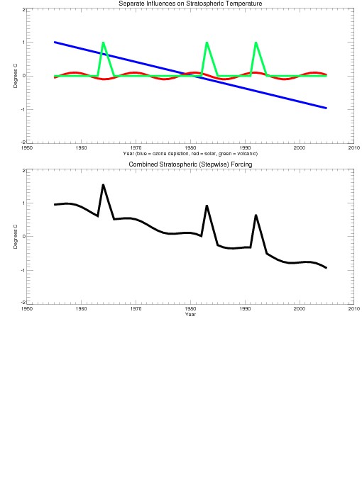
The attached diagram represents my understanding of the combined forcing factors described in the Ramaswamy paper "Anthropogenic and Natural Influences in the evolution of Lower Stratospheric Cooling."  They say that ozone depletion is a bigger factor than greenhouse gases.

My diagram should be compared with Figure 3.2b - Top on page 54 of "Chapter 3 Temperature Trends in the Lower Atmosphere" by Lanzante and Peterson.  You may have this file on your hard disk as sap1-1-final-chap3.pdf.

If I kind of squint, and defocus the lines, and mentally add some jitter, I can sort of see a stepwise behavior.  I just guessed at the relative amplitude of the 11-year solar cycle. Enjoy! Carl

---

Date: Thu, 1 Mar 2007 21:18:43 -0700 (MST)
From: Roger A Pielke Sr.
To: atoc7500
Subject: speaker tomorrow

Hi All, For tomorrow, the speaker for the first part of class will be Dr. DeZheng Sun on the IPCC models. This promises to be a very informatitive talk! Roger

---

Date: Fri, 02 Mar 2007 13:03:28 -0700
From: De-Zheng Sun
To: Roger A Pielke Sr.
Subject: Re: Guset Speaker - Dr. De-Zheng Sun

Dear Roger, Thanks again for the opportunity to talk with you and your class.  The papers from which I draw the bulk of the material for today's presentation are listed below. More information about my research can be found at  my web address <http://www.cdc.noaa.gov/people/dezheng.sun/>

Sun, D.-Z., T. Zhang, C. Covey,S. Klein, W.D. Collins, J.J. Hack, J.T. Kiehl, G.A. Meehl, I.M. Held, and M. Suarez, 2006 : Radiative and Dynamical Feedbacks Over the Equatorial Cold-tongue: Results from Nine Atmospheric GCMs J. Climate, 19, 4059-4074.

Zhang, T. and D.-Z. Sun, 2006 :Response of water vapor and clouds to El Nino warming in three NCAR models J. Geophys. Res.,111 , D17103, doi:10.1029/2005JD006700 .

Zhang, T., and D.-Z. Sun, 2006: Response of tropospheric water vapor and temperature to El Nino warming in four NCAR models. J. Climate, submitted.

Sun, D.-Z., J. Fasullo, T. Zhang, and A. Roubicek, 2003: On the Radiative and Dynamical Feedbacks over the Equatorial Cold-tongue. J. Climate, 16. 2425-2432

Pdf files for these papers can be downloaded at <http://www.cdc.noaa.gov/people/dezheng.sun/publications.shtml>, where you can  also find pdf files for recent papers about what drives El Nino events and how El Nino events  affect  the mean climate and the long-term heat balance.

The paper I mentioned in response to your question about why the percentage change of water vapor is more relevant is

Shine, K. P., and A. Sinha, 1991: Sensitivity of the earth's climate to height dependent changes in the water vapor mixing ratio. Nature, 354, 382-384.

Dr. John Fasullo, who worked with me some years ago, did a similar assessment, but with realistic cloud cover. Part of his work on this can be found at

Fasullo, J., and D.-Z. Sun , 2001: Radiative sensitivies to tropical water vapor under all-sky conditions. J. Climate, 14, 2798-2807.

It is a pleasure to talk with you and your class. Best wishes, De-Zheng

---

Date: Fri, 2 Mar 2007 14:01:00 -0700 (MST)
From: Roger A Pielke Sr.
Subject: Science funding

Hi All,  In response to the discussion today on science funding, below is information on this question.

Pielke, Jr., R.A., 2004. The End of Research? A Perspective for the Consortium for Science, Policy, and Outcomes, http://www.cspo.org, Arizona State University, October.
http://www.cspo.org/ourlibrary/perspectives/Pielke_October04.htm

Roger

---

Date: Sat, 3 Mar 2007 09:09:57 -0700
From: Marcia Wyatt
Subject: Bryden's MOC slowing questioned

Hi Everyone, I have attached a short article from Physics Today giving a critique of Bryden et al.'s assertion a couple of years ago that the MOC

was slowing (due to global warming). The author of this piece (Petr Chylek) notes an error in the use of Bryden's own data.

Chylek notes that he spoke directly with Bryden who stated that when he published the article in Nature, his original title had a question mark after the title, suggesting uncertainty in the conclusion. The editor of the journal insisted that question mark be removed... Enjoy. Marcia

---

Date: Sat,  3 Mar 2007 11:20:17 -0700 (MST)
From: Odele Malinda Hofmann
Subject: Re: Science funding

Hi Professor Pielke and class,

In class you suggested that science funding is up as well as funding for climate change research.  I didn't see this specific statement (re climate science) mentioned in your son's article.  Is there another article that addresses this statement directly?

What I did see in the article is that money spent on R&D has increased.  I, personally, have heard many statements, mainly in the news, that 3 select agencies have received increased funds for R&D.  These agencies are DOD (Department of Defense), DHS (Department of Homeland Security), and NASA.  The first 2 agencies are primarily defense related, and I don't think anyone would disagree that money spent on defense has increased substantially!  I have also read in the news that the majority of increased NASA funds is going towards Mars research and space exploration.  For these statements I am making, I have no hard articles or statistics to quote, but am just trying to portray a medley of information that I have garnered from magazines, newspapers, and television.

In addition, I would like to propose the suggestion that 'R&D' funding, does not distinguish between science funding or engineering funding.

Essentially, what I read in the article has still not convinced me that spending has increased for basic science research, or at least not in the areas of science research that I soon hope to have a career in.  Also, I do realize that this topic is not what our class is about.  It just piqued my interest, and I would appreciate more direct information related to funding in the atmospheric sciences. Best regards, Odele

---

Date: Sat, 03 Mar 2007 11:59:11 -0700
From: Laure M Montandon
Subject: Re: Science funding

Hi Odele and class, in the line of this discussion, I thought you might be interested in reading the following headline from the American Association for the Advancement of Science:

http://www.aaas.org/spp/rd/guihist.htm

Laure

---

Date: Sat, 3 Mar 2007 12:51:07 -0700
From: Jason English
Subject: Re: Science funding

I went straight to the facts - the federal budget (links below).   While it doesn't give the breakdown of spending within each department (which is

very relevant to whether atmospheric science gets its fair share of research) it does illustrate trends comparing one department to another.

$billions
Year   DOD  EPA  NASA  NSF   Science  Total   Science%
1992   287    4.0    14.0     2.2      20.2      1382      1.46%
2000   277    7.0    13.4     3.6      24.0      1790      1.34%
2006   419    7.6    16.5     5.6      29.7      2568      1.16%

One can look at these numbers in various ways.   Under both Clinton and Bush, Science spending has increased overall (but NASA was stagnant under Clinton; EPA under Bush).  However, Science is a tiny part of the total U.S. budget, and its percentage continues to decrease.  This decrease has accelerated under Bush to only 1.16% of our total budget, driven largely by increases of DOD spending.   I don't have the numbers here, but I understand that the current NASA budget is misleading because the money has been removed from earth-based science and is being transferred to Bush's focus on Mars.

2000-2006 http://www.whitehouse.gov/omb/budget/fy2006/tables.html
1992-2000 http://www.gpoaccess.gov/usbudget/fy01/pdf/hist.pdf

---

Date: Sat, 3 Mar 2007 14:12:13 -0700 (MST)
From: Roger A Pielke Sr.
Subject: Re: Science funding

Hi All, Please see the reply below from my son. Let me know if you feel a guest presentation on this subject would be valuable for you. Roger (Sr.)

You can share the below:

We just spent the past 3 weeks in my graduate seminar discussing US federal budgets for science and technology.  Here are a few thoughts:

*Overall R&D increased dramtaically through Clinton and Bush, and has now leveled off.  Looking at federal spending as a fraction of GDP is highly misleading.  The more appropriate metric is as a percentage of discretionary spending.

*Most of the increase has been for Defense (the "D" in R&D) and health (the "R" in R&D).

*Funding that is currently increasing is for NSF, NIST, and DOE science

*Climate research has been declining (slowly) since 1998 under Clinton and continuing under Bush.  Climate research currently receives about $1.8 billion per year, a bout half of which is for remote sensing programs in NASA.

*Climate technology research has been increasing and is projected to continue increasing.

*Only three agencies have a mandate to do "basic research" -- NSF, NASA, and DOE's Office of Science.  Climate research is not characterized as basic research.

I'd be happy to do a guest visit if there is interest to get into further details ...

---

Date: Sat,  3 Mar 2007 16:23:33 -0700 (MST)
From: Odele Malinda Hofmann
Subject: Re: Science funding

Hi Everyone! Wow.  Thanks for all this great information that's being sent along.  This will make for some very interesting reading. Even though I

started this email thread, I hesitate to request a guest speaker on the subject, just because it's not the primary purpose for our class.  Perhaps we could discuss it in next class, and see what everyone's view is? Again, thanks for passing along this information. Cheers, Odele

---

Date: Sat, 3 Mar 2007 17:27:56 -0700
From: Marcia Wyatt
Subject: Re: Science funding

This is all very good information. Thanks to all.

As Odele said, this is not the primary purpose for the class, but it is an important aspect. I agree that it might be something we all want to explore further.

I suggest a slightly different tact, though. I suggest that if we are interested enough to discuss the topic, despite its not being the primary purpose of the class, we might want to take the extra step and

have a speaker on the issue, so that our examination of its complexities can add to our knowledge base. An exchange of views only among ourselves might leave us feeling more informed than we actually are.  I suspect it is a rather time-consuming endeavor to scrutinize beyond the headlines. Importing comments on the topic from someone whose career is devoted to researching beyond the sound bites and editorials might give us a more complete and accurate outlook. I think we would be privileged to be exposed to the expertise.

Thanks again for all the information, and for broaching the topic in the first place. Marcia

---

Date: Sun, 4 Mar 2007 08:25:05 -0700 (MST)
From: Roger A Pielke Sr.
Subject: Re: Science funding

Hi Jason, Thank you for this analysis. My son has agreed to make a presentation to our class on this subject in our April 13th class. It is a subject that is appropriate for discussion and I am glad that you, Marcia and Odele have introduced this topic. Roger

---

Date: Sun, 4 Mar 2007 08:55:53 -0700 (MST)
From: Roger A Pielke Sr.
Subject: Friday class

Hi All,  Among the topics for Friday's class, I would like us to discuss the following:

1. Jason stated that the aerosol radiative forcing is better understood in the 2007 IPCC report compared with the 2001 IPCC Report. I will present the summary figures in the 2001 and 2007 SPMs and the state of science review in the 2005 NRC report to question this conclusion. Please come to class to present further evidence to support or refute my class (if you can place on powerpoint slides so we can show; if you send to Dallas, she can post on our class website).

2. Odele stated that we have a better understanding of the solar forcing of the climate system in the 2007 IPCC report than we did for the 2001 IPCC report. Please come to class to present further evidence to support or refute this conclusion. I will refer to the summary of the 2006 SORCE meeting on solar forcing at

http://www.climatesci.org/2006/09/20/354/

http://www.climatesci.org/2006/09/22/a-presentation-by-ra-pielke-sr-at-the-sorce-meeting-by-peter-pilewskie-entitled-an-overview-of-the-radiation-budget-in-the-lower-atmosphere/

http://www.climatesci.org/2006/09/25/overview-of-the-4th-annual-sorce-meeting-earths-radiative-budget/

http://www.climatesci.org/2006/09/27/overview-of-the-4th-annual-sorce-meeting-earth%e2%80%99s-radiative-budget-part-ii/

http://www.climatesci.org/2006/10/03/overview-of-the-4th-annual-sorce-meeting-earth%e2%80%99s-radiative-budget-part-iii/

http://www.climatesci.org/2006/10/25/2006-sorce-science-meeting-overview/

http://www.climatesci.org/2007/02/14/ocean-albedo-changes-resulting-from-variations-in-solar-radiation-a-newly-recognized-climate-forcing-and-feedback/

to support the view that we stll have a significantly incomplete understanding of this climate forcing. I also will ask one of the CU experts in solar forcing to present to our class in an upcoming week.

See you Friday! Roger

---

Date: Sun, 4 Mar 2007 09:12:09 -0700 (MST)
From: Pielke Roger A
To: Roger A Pielke Sr.
Subject: Re: Science funding

Hi All (from Roger Jr.)-

Jason, be caseful in any time series analysis of budgets that you adjust for the effects of inflation, so as to compare apples with apples over time.  Also, don't equate funding for a particular agency with funding for science, they are not the same thing.  And when looking at science as a part of the total budget you should really take out entitlements as these are growing faster than the budget as a whole and their inclusion will distort any analysis of relative trends.  The most comprehensive data on funding for R&D is kept by AAAS and can be found here:

http://www.aaas.org/spp/rd/guide.htm

The battle between human spaceflight and space science goes back almost 40 years in NASA, and presently has much more to do with the shuttle and station eating a very large part of the budget as NASA tries to start something new.

If any of you have specific questions on budget process or data, please email them before April 13th, meantime, have a look at my course page where we have just finished 3 weeks on the federal budget for R&D:

http://sciencepolicy.colorado.edu/about_us/meet_us/roger_pielke/envs5100/

Best regards, Roger (Jr.)

---

Date: Mon, 5 Mar 2007 07:30:18 -0700 (MST)
From: Roger A Pielke Sr.
Subject: paper on solar-climate influences

Hi All, Here is a new paper on solar-climate influences. I have not yet read to assess its value in this discussion.

Roger

Advances in Space Research (2007), doi: 10.1016/j.asr.2007.01.076
http://tinyurl.com/2tg3wm

Effect of Solar Variability on the Earth's Climate Patterns

Alexander Ruzmaikin
Jet Propulsion Laboratory, California Institute of Technology, Pasadena,
California

Abstract

We discuss effects of solar variability on the Earth's large-scale climate patterns. These patterns are naturally excited as deviations (anomalies) from the mean state of the Earth's atmosphere-ocean system. We consider in detail an example of such a pattern, the North Annular Mode (NAM), a wintertime climate anomaly with two states corresponding to higher pressure at high latitudes with a band of lower pressure at lower latitudes and the other way round. We discuss a mechanism by which solar variability can influence this pattern and formulate an updated general conjecture of how external influences on Earth's dynamics can affect climate patterns.

1. Introduction
The center of attention of this paper is the response of the Earth to solar variability on Space Climate time scales. In the context of Space Climate, the Earth can respond to solar variability on the 27-day solar rotation time scale, the 11-year solar cycle, the century scale Grand Minima, and even longer time scales. The shorter time scale effects are referred as Space Weather. Similar time scales discriminate the Earth's weather from the Earth's climate. Month-to-month and lower frequency variability on the Earth is considered to be climatic.

Observations, such as sunspot number records, indicate that the magnitude of solar variability increases from the solar rotation time scale to longer time scales. We can expect that in turn the Earth's responses become more pronounced with the increase of time scale. A transition from shorter to longer time scales implies averaging over small-scale atmospheric disturbances and the involvement of systems with more inertia than the atmosphere, in particularly the oceans.

Physical effects of solar variability involve either particles or irradiance. Here we discuss the responses to variations in solar irradiance. The solar cycle variations in total solar irradiance are small, 0.1%. However the magnitude of irradiance variations strongly depends on the wavelength and increases for the shorter wavelengths. Thus solar UV, which amounts to only a few % of the total irradiance, contributes 15% to the change in total irradiance (Lean, 2005). Solar UV mainly affects the stratosphere by creating and destructing ozone (in different parts of the atmosphere and at different wavelengths of radiation) and causing temperature changes. Effects of these changes on the underlying troposphere, where we live, depend on stratosphere-troposphere interactions. These interactions, as we show below, involve large-scale dynamical climate patterns. [...]

---

Date: Mon, 5 Mar 2007 08:31:48 -0700 (MST)
From: Roger A Pielke Sr.
Subject: Re: my class

Hi All, I have invited Dr. Peter Pilewskie of LASP to discuss solar climate forcings, and he has graciously agreed. He will present on April 20th and will send reading materials to us before hand. Roger

---

Date: Tue, 6 Mar 2007 10:53:16 -0700 (MST)
From: Roger A Pielke Sr.
Subject: Comprehensive Examination - Derek Brown (fwd)

Hi All,  Here is another very interesting and relevant (to our class) talk, Roger

Date: Tue, 06 Mar 2007 09:50:33 -0700
From: Laurie B. Conway
Subject: Comprehensive Examination - Derek Brown

COMPREHENSIVE EXAM - Derek Brown

Date and Time:  Monday, March 12 at 10:30am
Location:  CIRES/Ekeley Room S274

Title:  "Comparison of atmospheric hydrology over convective continental regions using isotope measurements from space"

Abstract:  The hydrologic regimes of convective continental regions involve complex balances of large-scale advective supply of water, surface exchange, and atmospheric condensation.  Measurements of the relative deuterium content in water vapor (delta-D) from the Tropospheric Emission Spectrometer (TES), combined with knowledge of isotopic fractionation theory, give a unique view of the dominant processes that contribute to regional differences in hydrology.  Results show that significant deviations from Rayleigh isotopic theory occur over tropical locations as a result of isotopic exchange within clouds. In addition, rainfall recycling signals are implicated through anomalously high delta-D values over the Amazon Basin, Congo River Basin, and northern Australian coastline.  A more refined understanding of the regional sources of water, by way of isotopic signals, may be used to add constraints to isotope-enabled Global Climate Models.

---

Date: Wed, 7 Mar 2007 09:01:10 -0700 (MST)
From: Roger A Pielke Sr.
Subject: Article from Journal of Climate (fwd)

Hi All,  Here is a new article (alerted to me by Dev Niyogi) that is relevant to our discussions of both the use of the global average surface temperature and in the use energy balance mode
Estimates of Uncertainty in Predictions of Global Mean Surface Temperature J. A. Kettleborough, B. B. B. Booth, P. A. Stott, and M. R. Allen

The abstract reads

"A method for estimating uncertainty in future climate change is discussed in detail and applied to predictions of global mean temperature change. The method uses optimal fingerprinting to make estimates of uncertainty in model simulations of twentieth-century warming. These estimates are then projected forward in time using a linear, compact relationship between twentieth-century warming and twenty-first-century warming. This relationship is established from a large ensemble of energy balance models.

By varying the energy balance model parameters an estimate is made of the error associated with using the linear relationship in forecasts of twentieth-century global mean temperature. Including this error has very little impact on the forecasts. There is a 50% chance that the global mean temperature change between 1995 and 2035 will be greater than 1.5 K for the Special Report on Emissions Scenarios (SRES) A1FI scenario. Under SRES B2 the same threshold is not exceeded until 2055. These results should be relatively robust to model developments for a given radiative forcing
history."

http://dx.doi.org/10.1175%2FJCLI4012.1

Roger

---

Date: Wed,  7 Mar 2007 15:13:33 -0700 (MST)
From: Carl Walther Drews
Subject: The drop is happening

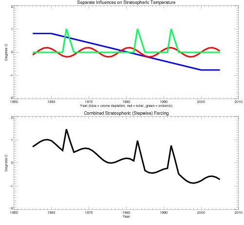
Regarding the stepwise cooling in the lower stratosphere, Jason and Josh pointed out that ozone depletion in the stratosphere is not completely linear, so I have modified my ozone depletion line to decrease only between the years 1960 and 2000 (just a wild guess).  Marcia also pointed out that anthropogenic aerosols in the upper troposphere should be enhancing the solar cycle there via solar heating, as the dirty tropopause absorbs more insolation.  The anthro aerosol effect should increase the amplitude of the solar cycle, which I have also done.  (Or maybe it should tilt up the ozone line at the end, which I have not done?)  The resulting "cartoon" graph is attached.

I found a web site containing stratospheric temperatures:
http://www.ghcc.msfc.nasa.gov/MSU/msusci.html

It's pretty hard to detect long-term signals visually in the raw data, but the download link also includes the 12-month running mean (yeah!).  So I plotted that in the second attached plot.

Dr. Pielke's prediction is correct; the temperature graph is going down at the end of the time series.  In other words, the (sinusoidal) solar cycle has again emerged from that pesky volcanic obfuscation.  The most recent solar peak is in 2003, which is right where my cartoon graph says it should be.

I have also attached the IDL script, in case anyone else wants to experiment.  Nobody loses - play until you win! Carl

---

Date: Thu, 8 Mar 2007 06:55:48 -0700
From: Marcia Wyatt
Subject: solar

Hi All, Friday I am going to give a presentation on solar forcing on climate. I am not an expert, by any means, but the topic has long fascinated me. In this "climate" of research, it is difficult to find ready access to this information. I will attempt to do the topic justice and weave together controversies regarding measurement, climate sensitivity to solar, and suggested possible mechanisms of amplification of the direct signal.

I have culled out of my stack of papers ones that I think would encapsulate the subject matter best. Not included in this set of attachments, but recommended, are ones already distributed; they include the Shindell 1999 paper, a few others I sent out along with that (should be under solar on class site), and the most recent Ruzmaikin paper forwarded to us by Dr. Pielke. There are many others, but these, together, provide a pretty good overview.

Svensmark 2007

VanLoon et al. 2006

Baldwin and Dunkerton 2004

Scaffeta and West 2005

See you tomorrow. Marcia

---

Date: Thu, 8 Mar 2007 08:06:16 -0700 (MST)
From: Roger A Pielke Sr.
Subject: Re: phone #: Land Use Science Steering Group Meeting (fwd)

Hi All, Here are two quite interesting papers on the reconstruction of long term temperature and in the biogeochemical role of CO2 in the climate system. Roger

Loehle, C., 2005: Estimating Climatic Timeseries From Multi-Site Data Afflicted With Dating Error pdf

Loehle, C., 2007: Predicting Pleistocene climate from vegetation in North America pdf

---

Date: Thu, 8 Mar 2007 14:38:05 -0700 (MST)
From: Roger A Pielke Sr.
Subject: House Hearing On Climate Science Issues

Hi All,  At some point, I would like us to discuss this March 7 2007 Hearing

Climate Change: Are Greenhouse Gas Emissions from Human Activities Contributing to a Warming of the Planet?
http://energycommerce.house.gov/cmte_mtgs/110-eaq.hrg.030707.Greenhouse_gas.shtml

Roger

---

Date: Fri, 9 Mar 2007 06:40:53 -0700 (MST)
From: Roger A Pielke Sr.
Subject: Friday March 9 2007 class

Hi All,  For today's class, Marcia and Jason will be giving presentations. Carl can also discuss further his stratospheric temperature model if needed. Afterwards, I want to discuss further the level of uncertainty on the

aerosol forcing and on the errors I claim to have found in the IPCC Report. The textbook for the class has finally arrived also, and I will be assigning a reading from it. See you shortly! Roger

---

Date: Fri,  9 Mar 2007 11:21:39 -0700 (MST)
From: Odele Malinda Hofmann
Subject: solar forcing papers

Hi All, Here are the papers I discussed today.  Dallas, would you please post to class website? Thanks, Odele

Y.-M. Wang, J. L. Lean, and N. R. Sheeley, Jr. MODELING THE SUN’S MAGNETIC FIELD AND IRRADIANCE SINCE 1713, The Astrophysical Journal, 625:522–538, 2005 May 20.

Lean et al., SORCE CONTRIBUTIONS TO NEW UNDERSTANDING OF GLOBAL CHANGE AND SOLAR VARIABILITY, Solar Physics (2005) 230: 27–53.

---

Date: Fri, 9 Mar 2007 12:37:54 -0700 (MST)
From: Roger A Pielke Sr.
Subject: Next Friday's class

Hi All, Marcia and Odele presented two excellent talks today! The associated discussion was very informative. (Marcia/Odele - please send your talks as pdfs to Dallas if that is okay with you and she will post on our weblog;

at the end the semester I plan to communicate the url for our class on Climate Science).

 For our next class, Jason will present a talk (and Carl will summarize a seminar that he attended). I will discuss the topics in the e-mail from earlier today, as well as start on Part III page 153-186 of the C&P book (please let me know if you cannot yet obtain it; check Climate Science for a 20% off by purchasing from the website directly to the publisher). Roger

Odele Coddington: An Overview of Sorce Contributions to New Understanding of Global Change and Solar Variability

Marcia Wyatt: The "Holy Grail" of Solar-Climate Research - Finding an Amplifying Mechanism

See accompanying notes for Wyatt ppt: PDF

---

Date: Fri, 9 Mar 2007 15:08:30 -0700
From: Marcia Wyatt
Subject: Re: Some CO2 stuff (in case you were wondering)

Hi all, Two things: I came across a "favorites" website address that I'd long forgotten about. It is a website to a list of abstracts/introductions of presentations to be given at a conference on

stratospheric-tropospheric coupling. The address follows for anyone interested. http://www.phys.ocean.dal.ca/people/po/Whistler.html

Secondly, I copied below a "snapshot" of the globe showing region of CO2 evasion from the ocean. The area of evasion is most pronounced in the cold tongues in both the Pacific and Atlantic basin. This is not representative of an El Nino year, and this time of year coincides with the seasonal diminishment of southeasterlies, so the effect of evasion is less pronounced in the eastern section than it is when upwelling is stronger. But you can see evasion (red and yellow areas) occurs all along the equatorial upwelling region.

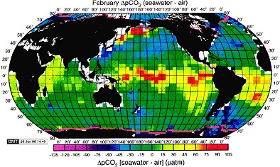
I asked my advisor about the CO2-uptake/temperature issue. He agreed that, perhaps counterintuitively, the cold tongue, especially during La Nina, delivered more CO2 to the atmosphere than any other oceanic region, and that
amount is quite large. But he added that while the ocean is the source of CO2 (due to the saturation pressure (developed from oxidation of dissolved organic matter in deeper waters)), there is, indeed, elevation of CO2 during
El Ninos, as well. The difference is that during El Ninos, the source is terrestrial, not oceanic. This is due to the supposed greater number of wildfires that ignite during an El Nino event. So, depending on the impact on the terrestrial biosphere during an El Nino, the indirect CO2 delivery to the atmosphere might be greater during these warm events.

I also asked about the cold temperatures as far as the amplified solubility factor; he stated that cold temperatures in the high latitudes of the oceans plays more of a role than it does in low latitudes, as seasonality is strong there, so winter temperature plays more of a role in amplifying CO2-drawdown at high latitudes than in the low latitudes. In the case of the tropics, seasonality does not exist (as far as temperature goes), so the saturation pressure dominates as the critical change in conditions.

But (and finally) there is another complicating factor. I alluded to it today. It is called the Revelle factor. It is a chemical aspect that competes with this temperature related solubility factor. In fact, areas of warm water in the tropics tend to have an advantage over the cool high latitudes in the uptake of CO2, at least in the summer months when the high latitudes are less cold. It has to do with the fact that CO2 "leaks" out with warmer temperatures (away from cold tongue), and changes the chemistry. It changes it in such a way that something called the carbonate alkalinity goes up. This makes CO2 uptake more likey in these warm waters than in the relatively cooler, less carbonate-rich waters.

Not straight-forward, that's for sure!....More than you ever wanted to know likely, but just in case you couldn't get to sleep wondering about it :-)... Marcia

---

Date: Sat, 10 Mar 2007 16:27:19 -0700 (MST)
From: Roger A Pielke Sr.
Subject: Channel 4 news show

Hi All,  There is a TV show discussion of solar forcing, as well as on the IPCC process (its a long show). If we have time, we can discuss the

climate science that they present (in terms of where we agree and where we disagree).

http://video.google.com/videoplay?docid=9005566792811497638&q=The+Great+Global+Warming+Swindle&hl=e

We can also do that with the other TV documentaries that have appeared as well as Al Gore's movie.

e.g.

http://www.hbo.com/docs/programs/toohot/?ntrack_para1=leftnav_category5_show1

http://www.climatesci.org/2006/07/07/nbcdiscovery-channel-show/

Roger

---

Date: Sun, 11 Mar 2007 12:42:17 -0600
From: Marcia Wyatt
Subject: pdf of ppt

Hi Everybody, I have attached the pdf of the solar ppt plus a separate document with the copied notepages for given slides.

Please note on slide 12 of the ppt I have added information. This was the slide of Solanki '04's C-14 curve that I poorly explained. I re-read the caption. As I now understand it, the trend in C-14 was

trending downward throughout much of the Holocene due to an increasing geomagnetic field, but within the last 1500 years, the field has been strongly decreasing (upswing in curve; this is the part I stumbled over.). This is shown by the red line, on which an undulating black line, representing solar variability, is superimposed.

If I've failed to explain anything or if you detect errors, please let me know. Marcia

The "Holy Grail" of Solar-Climate Research - Finding an Amplifying Mechanism

See accompanying notes for Wyatt ppt: PDF

---

Date: Tue, 13 Mar 2007 09:30:21 -0600
From: Marcia Wyatt
Subject: aerosol article

Hi Everybody, I just came across this one page synopsis in Science of some modeling studies with aerosols, revealing alterations of oceanic and atmospheric circulation patterns that researachers

say resemble observations. It's a quick and interesting read. Marcia

---

Date: Tue, 13 Mar 2007 19:14:13 -0600 (MDT)
From: Roger A Pielke Sr.
Subject: a paper relevant to solar forcing

Hi All,  Here is a paper I would like us to discuss Friday or on Monday (don't forget our make class at 8am in the Stadium. This is a make-up for Friday the March 23rd class.

Ellis et al. 1978: The annual variation in the global heat balance of the Earth. J. Climate. 83, 1958-1962
http://www.climatesci.org/publications/pdf/ellis%20et%20al%20JGR%201978.pdf

Also, please e-mail all of us the status of your class project. Roger

---

Date: Wed, 14 Mar 2007 11:45:30 -0600
From: Jason English
Subject: Jason's Project

Regional Climate Change due to Aerosols by Jason English

I am going to be using NCAR's Community Atmosphere Model (CAM) to model the effects of Aerosols on regional climate, specifically in regions outside of the aerosol perturbation.   The article that Marcia sent highlights the
possible climatic impacts that Asian Aerosols can have on other regions (e.g. NW Australia). I may conduct a similar study to understand whether CAM shows a similar result, or I may focus on a different region (TBD).

Aerosols are produced naturally and anthropogenically, and their spatial distribution varies significantly. Aerosols affect climate by absorbing and/or scattering shortwave and/or longwave radiation.   Depending on the altitude, concentration, location, and composition, aerosols may cause a cooling or warming effect on regional climate.    In regions with high concentrations of aerosols, the radiative forcing may be very high. Additionally, aerosols may cause changes in atmospheric circulation which can alter climate in regions distant from the source.

---

Date: Wed, 14 Mar 2007 13:00:20 -0600 (MDT)
From: Dallas Staley
Subject: pdf of Roger's Presentation for Friday

The pdf of this presentation will be posted on the website with this email.

Overview of Global Climate Forcings and Feedbacks by Roger A. Pielke Sr., March 16, 2007

---

Date: Thu, 15 Mar 2007 09:36:29 -0600
From: Laure M Montandon
Subject: EOS discussion on climate models validity

Hi all, I just got the March 6th EOS in my mailbox, and I found the following discussion on climate models validity that I thought was interesting.

I will present an overview of the arguments presented in this article on Monday, March 19th during class. Laure

---

Date: Fri, 16 Mar 2007 15:26:08 -0600 (MDT)
From: Roger A Pielke Sr.
Hi All,  Here is the debate that went on in New York this week.

http://www.intelligencesquaredus.org/TranscriptContainer/_GlobalWarming-edited%20version%20031407.pdf

I much prefer the weblog format to exchange scientific views. There will soon be a podcast of this posted, as I understand. Roger

---

Date: Fri, 16 Mar 2007 14:06:53 -0600 (MDT)
From: Roger A Pielke Sr.
Subject: Monday's class is at 8am in the Stadium

Hi All, Thank you for two excellent presentations today! Jason's overview of aerosol radiative forcing was the best I have ever heard! On Monday, Laure will present, and I will go over Chapter 8. We will also review the urls that have recently been posted on the class website.

Enter Gate #7 and go the ATOC area on the second floor. We will meet in one of the Conference rooms there.

Regional Climate Change due to Aerosols by Jason English

Lower Stratospheric Cooling and Abrupt Change in Arctic Sea Ice by Carl Drews

Have a good weekend! Roger

---

Date: Fri, 16 Mar 2007 20:40:42 -0600
From: Laure M Montandon
Subject: BBC E-mail: Caution urged on climate 'risks'

"Fresh" on the BBC news website:

** Caution urged on climate 'risks' **
Two leading UK climate researchers say "overplaying" the global warming message risks confusing the public.
< http://news.bbc.co.uk/go/em/fr/-/2/hi/in_depth/6460635.stm >

Laure

---

Date: Mon, 19 Mar 2007 12:10:25 -0600 (MDT)
From: Carl Walther Drews
Subject: Carbon dioxide increase leading temperature increase

ATOC 7500-002:

Here is the figure I mentioned in class today, where the CO2 increase happens _before_ the increase in temperature.  Note that historical time proceeds from right to left.

The citation is: “Eight glacial cycles from an Antarctic ice core”, by EPICA community members (Eric Wolff is the lead author), pages 623-628.  Nature volume 429, 10 June 2004.

The graph shows Termination V at 425 kya.  Event 1 = peaks reached.  Event 2 = start of the increase.  The time scale here runs from 415.5 kya to 443 kya.  The total span of the graph is 27,500 years. deltaD is a temperature proxy.

EPICA is still plowing through the ice core.  We'll have to wait to see what the other major transitions look like.

Carl

---

Date: Mon, 19 Mar 2007 13:02:28 -0600 (MDT)
From: Roger A Pielke Sr.
Subject: class materials

Hi All, Thank you Laure for another excellent talk!

Laure Montandon, 2007: How reliable are climate models? A review of a recent EOS discussion.

For readings over our break, please look at:

1. RE: nitrogen deposition

Lamarque J.-F., et al. (2005), Assessing future nitrogen deposition and carbon cycle feedback using a multimodel approach: Analysis of nitrogen deposition, J. Geophys. Res., 110, D19303, doi: 10.1029/2005JD005825
http://www.agu.org/pubs/crossref/2005/2005JD005825.shtml

[see also
http://www.climatesci.org/2006/02/02/further-evidence-of-the-role-of-nitrogen-deposition-as-a-first-order-climate-forcing/


2. RE: black carbon deposition
Hansen, J., and L. Nazarenko 2004. Soot climate forcing via snow and ice albedos. Proc. Natl. Acad. Sci. 101, 423-428, doi:10.1073/pnas.2237157100.
http://dx.doi.org/10.1073/pnas.2237157100

3. RE: Lags in the Climate System
see http://www.climatesci.org/2006/06/27/lags-in-the-climate-system/

4. RE: Issues with the Surface and Tropospheric temperature reconciliation

Pielke Sr., Roger A., 2005: Public Comment on CCSP Report "Temperature Trends in the Lower Atmosphere: Steps for Understanding and Reconciling Differences". 88 pp including appendices.
http://www.climatesci.org/publications/pdf/NR-143.pdf

CCSp Report "Temperature Trends in the Lower Atmosphere: Steps for Understanding and Reconciling Differences"
http://www.climatescience.gov/Library/sap/sap1-1/finalreport/default.htm

4. Chapters 4-7 in the book. This is on "Inadvertent human impacts on regional weather and climate" with the chapter headings

i) Anthropogenic emissions of aerosols and gases

ii) Urban-induced changes in precipitation and weather

iii) Other land-use/land-cover changes

iv) Concluding remarks regarding deliberate and inadvertent human impacts on regional weather and climate

Also, please e-mail the progress on your class projects to everyone. Also, let me know which of the two dates (April 27th or May 4) that you would like to present.

Tomi will be presenting a talk to our class when we return. Have a great Spring break! See you on April 6th. Roger

---

Date: Mon, 19 Mar 2007 14:43:41 -0600 (MDT)
From: Joshua Aaron Mc Grath
Subject: Carbon Monoxide Chemistry

Hi all, I looked up some of the atmospheric chemistry pathways involving carbon monoxide. The primary loss of CO in the atmosphere is oxidation to carbon dioxide by reaction with the hydroxyl radical, OH. Carbon monoxide will also react more readily with OH than other common atmospheric constituents, such as methane and ozone. Therefore, carbon monoxide is an indirect radiative forcer through its oxidation pathway as well as keeping OH from reacting with other greenhouse gases, particularly methane. Josh

---

Date: Mon, 19 Mar 2007 14:49:28 -0600
From: Jason English
Subject: Re: Carbon Monoxide Chemistry

Here is an article which supports what Josh found.    It also says that CO has a lifetime of about 2 months which is long enough to make CO a good tracer.

http://www.sciencedaily.com/releases/1999/12/991220153123.htm

---

Date: Mon, 19 Mar 2007 15:36:01 -0600
From: Jason English
Subject: Nitrogen, Sulfur emissions

Primary source of NOx emissions: transportation
Primary source of SOx emissions: power plants

A typical catalytic converter is capable of destroying around 98 percent of NOx (and hydrocarbons and CO) produced by the car's engine.  However, transportation remains the most significant contributer to NOx emissions (~50% of emissions in the U.S.) because:

1. Catalytic converters aren't always operating at their ideal environmental conditions.
2. The sheer quantity of combustion occuring in automobiles adds up
3. Some transportation doesn't have catalytic converters (e.g. construction equipment)

From a biogeochemistry standpoint, global NOx emissions amount to ~17 Tg annually.  Compare this to fertilizer consumption which amounts to 80 million tons annually (353 Tg if my calculation is correct).  So from a global biogeochemistry standpoint, fertilizer adds an order of magnitude more nitrogen to the soils than NOx emissions.   However, fertilizer isn't as mobile so NOx emissions could taint remote forested regions that fertilizer wouldn't reach.

And finally, sulfur is removed from gasoline in most countries before it reaches the gas pump due to pollution laws.  Therefore, the primary source of SOx into the atmosphere is due to power plants, rather than transportation.   (Transportation is only 2% of total SOx emissions)

References:
Catalytic Converters  http://www.webwire.com/ViewPressRel.asp?aId=27293
NOx emissions sources  http://www.epa.gov/air/oaqps/bluebook/noxsrc93.html
Fertilizer consumption http://interactive.usask.ca/Ski/agriculture/soils/soilfert/soilfert_cons.html
GEIA inventory for NOx, SOx emissions http://www.geiacenter.org/presentData/nox.html

---

Date: Mon, 19 Mar 2007 17:41:44 -0600
From: Marcia Wyatt
Subject: Re: Carbon dioxide increase leading temperature increase

Hi All, Thanks Carl for that figure.

I quickly read the accompanying article. In my cursory review, I did not find any support for the correlation. They do mention a modeled time-lag (I'll explain below) and the say they "expect" that the pairs (referring to the T proxy and CO2 values) to be "roughly synchronous", and they also say that, as with the previous four terminations, the CO2 and T vary synchronously. That statement has

no reference and it contradicts an article I have attached on one of the terminations referred to. This article was referred by the Real Climate web site. I have also attached a document
copied from that dialogue on Real Climate discussing the basis for the T, then CO2 lag (which is, without question, a positive feedback in these glacial terminations, but not the initiator (which says nothing about today's climate)). Basically, problems of low accumulation coupled with the fact that ice is always older than the air bubbles it encases (as much as a thousand years or more in Antarctica), complicate the pinpointing of relative timing. But, to my knowledge, there is only small debate about the lag. It is considered to be reflective of the overturning circulation ramping up preceding a glacial termination, thus "spilling" out CO2 from old, deep water. And, as an aside, at these terminations, there is a bi-polar, out-of-phase temperature pattern b/n the Arctic and the Antarctic. This phasing can even be seen on centennial scales now with the newest Vostok core, out last fall. So, beware of how the graphs "read".

In addition to the two attachments concerning this lead-lag topic, I have attached a document I compiled that describes CO2/climate relationship in the Eocene and Miocene. It simply amplifies the point that climate forcing involves more than one factor. (I copied three different excerpts from different pages, so it doesn't "flow".)

And finally, I have attached an excerpt from something Lindzen sent me. It is about water vapor and what he feels is an incorrect understanding about the Clausius-Clapyeron relation. This is out-of-my immediate field of study, but this man's knowledge on the topic of water vapor is quite stellar. Interestingly, Lindzen was the advisor of  Dr. Sun, who spoke to us a few weeks ago.

Caveat, as always: I'm not an expert on anything (except maybe sleeping), but on the information provided here, I'm not uncomfortable. I think it is all correct, but please point out errors if you find them.

M

---

Date: Mon, 19 Mar 2007 18:18:46 -0600 (MDT)
From: Roger A Pielke Sr.
Subject: Re: Carbon dioxide increase leading temperature increase

Hi Marcia,  Thank you for keeping up this discussion! On all of the subjects, please keep up the momentum of debating the science. Dallas will post on the class website to keep us documented.

Roger

---

Date: Mon, 19 Mar 2007 21:06:09 -0600
From: Marcia Wyatt
Subject: Re: one more thing on the mechanism

One more thing...(sorry). I should have added one more thought on the mechanism: to make it more clear.

Obliquity changes are suspected to have perturbed the ocean-atmosphere system, causing warming and a rejuvenation of the meridional overturning circulation (aka thermohaline circulation); then,

the CO2 was delivered in lagged response.

---

Date: Tue, 20 Mar 2007 13:29:15 -0600 (MDT)
From: Tomislava Vukicevic
Subject: On models and observations

I am sorry I again missed good discussion. Glad for continuation via e-mail!

Since I'll have presentation in the class on "Integrating models with observations" I am sending as starter on the general subject a recent commentary by one of my favorite authors in my expertis

area (inverse modeling and data assimilation in geosciences).

"It is harsh world for the modelers and there is no insurance company to cover the losses"

Tomi

---

Date: Wed, 21 Mar 2007 21:04:18 -0600 (MDT)
From: Roger A Pielke Sr.
Subject: suggested class calculation

Hi All,  As has been discussed on the Climate Science weblog by Issac Held and,Gavin Schmidt, they claim that the global averaged evaporation does not have to equal the globally averaged precipitation. I disagree, as over a,long enough time period, the two must be nearly equal even if there is,more water in the atmosphere from the increased evaporation (i.e. a,constant relative humidity).

To answer this question quantitatively, I would like you to

1. obtain an estimate of   the current global average evaporation in kilograms/year.

2. obtain the current mass of water in the atmosphere in kilograms.

3. Assume a 5% increase in the evaporation rate (kg per year), what is the fractional change this would cause in the mass of water in the atmosphere assuming there is no increase in precipitation.

I would like to discuss this in class on April 6, but please also e-mail among us before then.

Roger

---

Date: Thu, 22 Mar 2007 16:08:46 -0600 (MDT)
From: Carl Walther Drews
Subject: Carbon dioxide and temperature in Antarctic ice cores

(one more try at sending this . . .)

Marcia and all - You're right, the lead-lag relationship between temperature and CO2 in Antarctica cannot be simply deduced by graphing them both vs. the depth at which they were measured. The problem is in how the ice cap forms and packs.  A snowflake gets locdked into the ice matrix pretty quickly, so we can trust the Oxygen isotopes to be from that level (said Scott Gregory at his Comps 2 yesterday).  But the ice takes a while to pack, especially during low accumulations like at Dome C in Antarctica.  During the packing time, the upper layers of snow can communicate with the atmosphere via diffusion.  So newer air (Argon and CO2) can seep down into the older snow (the firn layer) before the final compaction.

The Caillon article that Marcia attached explains all this, using Vostok Termination III at 240 kya.  I have attached their Figure 1, showing deuterium (a water-based temperature proxy) on the top and Argon isotopes (a gas-based temperature proxy) on the bottom.  Argon is useful because there is no known way it can force temperatures.  Next the researchers skooched over the Argon curve until it matched deuterium, producing a shift of 4100 +- 250 years between ice and the gas bubbles trapped in it.  When they shifted the CO2 curve over by the same amount, they found that CO2 lagged temperature by 800 +- 200 years.  More details are in the article.

They postulate the following sequence:
Time 0 years: Antarctica gets warmer due to orbital forcing.
Time 800 years: Change in ocean circulation leads to rise in carbon dioxide.
Time 5,000 years: Northern Hemisphere de-glaciates, prompted by CO2 amplification of the original orbital forcing.

---

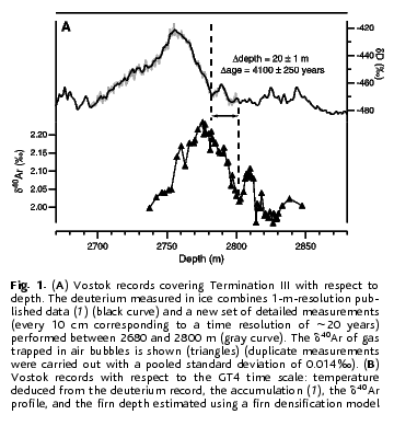
Date: Thu, 22 Mar 2007 16:19:56 -0600 (MDT)
From: Carl Walther Drews

And if you want to look at some MOPITT data, here is the site: http://gctm.acd.ucar.edu/intex_support/forecast_maps.shtml

Those graphical displays are courtesy of Louisa Emmons and (ahem) me.

Carl

---

Date: Fri, 23 Mar 2007 12:21:19 -0600
From: Laure M Montandon
Subject: suggested class calculation - my attempt

Hi All, so I tried to come up with a rough estimate of my own. I have no idea if that is even realistic. So please tell me if I got something wrong.

I found some numbers for my estimate in: Quante M, Matthias V, Water in the Earth's atmosphere
<http://apps.isiknowledge.com/WoS/CIW.cgi?SID=4ACE7c1gEBDcEC55O7h&Func=Abstract&doc=3/7>
JOURNAL DE PHYSIQUE IV 139: 37-61 DEC 2006

I attached the paper for info. I used the values from the following tables

*Amount of water in the atmosphere:*
12,900 km3 = 12.9x10^15 kg
Note that this estimate is based on data from 1996 or earlier. Not sure how it was estimated, but my guess is that it is possible to find more recent estimates somewhere.

*Estimate of global average evaporation:* I used the values from the Trenberth et al. paper (2006).

433x10^15 kg evaporation over ocean
62x10^15 kg evaporation over land
TOTAL = 495x10^15 kg
*
Increase of 5% of ocean evaporation (I left the land one constant):
*Add 433x0.05x10^15 kg = 21.65x10^15 kg

*If precipitation remains constant, this means that the new water content in the atmosphere is:
*34.55x10^15 kg, i.e. more than twice its original content (2.6 times more)

On the other hand, if we keep the water content in the atmosphere constant, and assume all the added water goes into precipitations, then the increase of precipitation is only of 4.4%.

Does that sound reasonable? Laure

---

Date: Fri, 23 Mar 2007 15:35:50 -0600 (MDT)
From: Joshua Aaron Mc Grath
Subject: Webcast about Antarctic Ice Sheets and Global Warming

Hi everyone, I don't remember seeing any emails about this webcast so thought I would pass this along.

Next Wednesday , March 28, at 7 pm CST the University of Texas, Austin will be hosting Dr. David Vaughan, PI for the British Antarctic Survey Core Program: Glacial Retreat of Antarctica and Deglaciation of the Earth System (GRADES). He will be discussing how global warming affects Antarctic ice sheets and global sea level as well as other aspects of climate change.
The link for the webcast as well as more information about the talk is below.

http://www.esi.utexas.edu/outreach/ols/lectures/Vaughan/

Josh Mcgrath

---

Date: Fri, 23 Mar 2007 16:48:10 -0600 (MDT)
From: Roger A Pielke Sr.
Subject: Re: suggested class calculation - my attempt

Hi Laure, This is an effective analysis and a very good reference paper. On the 4.4% increase in precipitation, I assume this is because the evaporation from both ocean and land increased by 4.4% (the 5% you list is for the ocean part).
 On the increase in the new water content of the atmosphere(without an increase in precipitation), what time period is this for? [the evaporation is a flux and the atmosphere is the reservoir). The reservoir would, of course, continue to increase in amount with precipitation held constant.

I look forward to more discussion on this very interesting topic! Roger

---

Date: Sun, 25 Mar 2007 12:08:58 -0600
From: Laure M Montandon
Subject: Re: suggested class calculation - my attempt

Hi all, Sorry, I forgot to mention the time period, it is over a year. I computed the increased precipitation as follow:

*Amount of water in the atmosphere:*
12,900 km3 = 12.9x10^15 kg

*Estimate of global average evaporation per year:*
495x10^15 kg/a

=> in order for the amount of water in the atmosphere to remain constant, the amount of water that is precipitated every year is:
495x10^15 - 12.9x10^15 = 482.1x10^15 kg/a

Comparing this with a 5% increase in evaporation over the oceans (i.e. 21.65x10^15 kg/a added to the atmospheric water), this would increase the overall precipitation by 4.5% (21.65/482.1) over a year. It is not quite 5%, as Dr Pielke mentionned, as the evaporation over land is estimated to remain constant.

Laure

---

Date: Mon, 26 Mar 2007 06:56:32 -0600 (MDT)
From: Roger A Pielke Sr.
Subject: Re: suggested class calculation - my attempt

Hi Laure, Thank you for the follow up! Roger

---

Date: Mon, 26 Mar 2007 07:00:35 -0600 (MDT)
From: Roger A Pielke Sr.
Subject: another issue to discuss on April 6th

Hi All, We have already discussed the conclusion that the net radiative feedbacks must be negative IF the 2007 IPCC SPM are correct and IF the recent ocean heat content changes are accurate. I posted this on Climate Science
http://www.climatesci.org/2007/03/19/climate-feedbacks-must-be-a-negative-effect-on-the-global-average-radiative-imbalance-if-the-ipcc-conclusion-of-anthropogenic-radiative-forcings-are-correct/

Please be prepared to further discuss this hypothesis that the net radiative imbalance is less than the net radiative forcing (i.e., the real climate system has a muted global warming response to anthropogenic forcing). Roger

---

Date: Mon, 26 Mar 2007 13:44:24 -0600 (MDT)
From: Carl Walther Drews
Subject: Evaporation and precipitation

From the textbook "Meteorology Today", by C. Donald Ahrens, Sixth Edition, 2000; pages 108-109: "In all, evaporation and transpiration from continental areas amount to only about 15 percent of the nearly 1.5 billion billion gallons [sic] of water that annually evaporate into the atmosphere; the remaining 85 percent evaporates from the oceans.  If all of this vapor were to suddenly condense and fall as rain, it would be enough to cover the entire globe with 2.5 centimeters, or 1 inch of water.*"

"*If the water vapor in a column of air condenses and falls to the earth as rain, the depth of the rain on the surface is called precipitable water."

Based on Laure's calculation and a few other web sites:
http://www.geocities.com/CapeCanaveral/Hall/5606/hydro/verdamp.htm
http://www.geo.cornell.edu/eas/education/course/descr/EAS201/Site/Lecture%20Notes_files/Chapter%209-11RR-2006.JPM.pdf

I think the Ahrens textbook should say, "0.15 billion billion gallons".  With that correction, the paragraph above tells us the answers to Roger's questions 1 and 2.

1.  Current global average evaporation = 0.15 billion billion gallons
= 1.5e17 gallons * 3.7854 liters / 1 gallon
= 5.7e17 liters * (1 kilogram / 1 liter)
= 5.7e17 kilograms annually

2.  Current mass of water in atmosphere
= 2.5 centimeters * surface area of earth
= 2.5 cm * 4 * pi * 6367^2 km^2
= 1.27e9 cm km^2
= 1.27e13 m^3
= 1.27e16 kilograms

The annual evaporation rate is 45 times the amount of water in the atmosphere at any instant.  This result implies that the average lifetime for water vapor is about 8 days.

3. A 5% increase in the evaporation rate would be:
= 5.7e17 * 0.05 = 2.85e16 kilograms more annually

For the atmosphere to "hold" that much more water, it would have to hold 2.85e16 / 1.27e16 = 2.2 times more water than it holds now.

That change would make it pretty cloudy. Carl

---

Date: Mon, 26 Mar 2007 14:06:58 -0600 (MDT)
From: Carl Walther Drews
Subject: Australian project statusMy high school friend JB Friday is a Professor of Forestry at the University of Hawaii.  He recommends treating pre-human Australia as a "dry forest", as opposed to a "wet forest" like the Amazon jungles.  He says that slash-and-burn publications will probably be more useful than forest fire publications.  As a starting point, I can use estimates of 100 to 200 t/ha biomass and have my Aborigines combust 60% to 80% of that.

Carl

---

Date: Mon, 26 Mar 2007 19:08:54 -0600 (MDT)
From: Roger A Pielke Sr.
Subject: Re: Evaporation and precipitation

Hi Carl (and Laure) Thanks for following up on this question. It certainly appears that the observation of no increase in global average precipitation is consistent with a zero increase in global average evaporation.

Since it is an evaporation increase that is required to amplify the positive radiative forcing from CO2 (from the water vapor feedback (from higher SSTs)), this raises issues with the existance of higher atmospheric water vapor as claimed in the 2007 IPCC SPM (which if true would have to occur for other reasons than "global warming"; perhaps an aerosol effect). It raises issues on this aspect of the statements by Gavin Schmidt and Issac Held on Climate Science.

Please keep the comments coming! Roger

---

Date: Tue, 3 Apr 2007 09:45:09 -0600 (MDT)
From: Roger A Pielke Sr.
Subject: Re: Friday class

Hi All, For Friday, Tomi is giving a presentation (Tomi - please send us any material to read). Also, afterwards, we will discuss the precipitation/evaporation issue and a summary of the land-use/land-cover meeting that I am attending this week. We can also discuss the implications of the new Supreme Court ruling on CO2. Roger

---

Date: Wed,  4 Apr 2007 08:41:40 -0600 (MDT)
From: Tomislava Vukicevic
Subject: April 6th class reading material

Atatched is reading material for the Friday class related to my short presentation on "Integrating Models and Observations-Data assimilation/Inverse Modeling"

The first file "Introduction ..." is part of my lecture notes. Other two are recent articles which speak about 1) utility of satellite observations in variety of modeling (Making the Most of Earth Observation with Data Assimilation by O'Neill et al. ) and 2) need for and means of data assimilation in biogeoscience modeling (Marine geochemical data assimilation in an efficient Earth System Model of global biogeochemical cycling by Ridgewell et al.) .

Intended discussion topic is "Assessing and reducing model errors"

Tomi

---

Date: Wed,  4 Apr 2007 16:26:20 -0600 (MDT)
From: Carl Walther Drews
Subject: It's not our fault!

According to a recent study, Mars is experiencing global climate change:

http://www.cnn.com/2007/TECH/space/04/04/mars.climate.reut/index.html

They say dust storms are causing a change in the Martian planetary albedo, and melting the southern polar ice cap.  The original article is in Nature. Carl

---

Date: Wed, 4 Apr 2007 17:31:46 -0600 (MDT)
From: Roger A Pielke Sr.
Subject: Re: It's not our fault!

Hi Carl,  Thanks! We should discuss this on Friday too. Roger

---

Date: Thu, 5 Apr 2007 13:17:39 -0600 (MDT)
From: Roger A Pielke Sr.
Subject: More on the water vapor issue

Hi All,  A comment on my weblog alerting me to a trend analysis of water vapor trennds is very interesting. We will discuss tomorrow.

http://www.cdc.noaa.gov/cgi-bin/Timeseries/timeseries.pl?ntype=1&var=Specific+Humidity+%28up+to+300mb+only%29&level=300&lat1=90&lat2=-90&lon1=-180&lon2=180&iseas=1&mon1=0&mon2=11&iarea=0&typeout=2&Submit=Create+Timeseries

Roger

---

Date: Thu, 05 Apr 2007 15:01:53 -0600
From: Laure M Montandon
Subject: Fungi are affected by climate change according to Science

Hi all, here is a short entertaining read (you can see the full article in Science) http://news.bbc.co.uk/2/hi/science/nature/6524013.stm

Full article: http://www.sciencemag.org/cgi/content/abstract/316/5821/71?maxtoshow=&HITS=10&hits=10&RESULTFORMAT=&fulltext=Alan+Gange&searchid=1&FIRSTINDEX=0&resourcetype=HWCIT
Laure

---

Date: Thu, 05 Apr 2007 15:30:51 -0600
From: Laure M Montandon
Subject: Seminar next Monday on sea level change

INSTAAR NOON SEMINAR
Monday, April 9th, Noon-1pm
Room 620, RL-3
R. Steven Nerem
NCAR

Satellite Measurements of Sea Level Change

Over the last few decades, satellite geodetic measurements together with in situ measurements, have revolutionized our understanding of present-day sea level change. With measurements from satellite altimeter missions and satellite gravity missions, we are now able to start answering some important questions with regards to global sea level
change and its regional variations. What have we learned from these measurements? Would we change any of the decisions we made in the past? What are the remaining questions to be answered? What suite of measurements are needed to answer these questions? The record of sea level change from satellite altimetry will be reviewed, its error sources and limitations discussed, and the results placed in context with other estimates of sea level change from tide gauges, in situ measurements, and global climate models. The much shorter, but just as important, record of ocean mass variations from satellite gravity measurements will be similarly reviewed. Finally, the need for
continuing the satellite measurements of sea level change, and possibly developing new measurements, will be discussed in the context of future missions and the scientific gain that would result.

---

Date: Thu, 5 Apr 2007 16:11:35 -0600
From: Jason English
Subject: Re: More on the water vapor issue
Parts/Attachments:
1 OK 112 lines Text (charset: ISO-8859-1)
2 Shown 118 lines Text (charset: ISO-8859-1)
----------------------------------------

Interesting. Does anybody know how the NOAA plot NCEP reanalysis was conducted? Which observations, whether the differences are statistical, etc? I found an article published last year which conducted a global assessment from 1976-2004. The authors found global RH to remain constant over the time period but specific humidity to increase alongside temperature (statistically sig. in the NH, not statistically sig in SH).

Title: Recent climatology, variability, and trends in global surface humidity
Author(s): Dai AG (Dai, Aiguo)
Source: JOURNAL OF CLIMATE 19 (15): 3589-3606 AUG 2006
Document Type: Article
Language: English
Cited References: 59 Times Cited: 2 Find Related Records Information
Abstract: In situ observations of surface air and dewpoint temperatures and air pressure from over 15 000 weather stations and from ships are used to calculate surface specific (q) and relative ( RH) humidity over the globe (60 degrees S - 75 degrees N) from December 1975 to spring 2005. Seasonal and interannual variations and linear trends are analyzed in relation to observed surface temperature ( T) changes and simulated changes by a coupled climate model [ namely the Parallel Climate Model (PCM)] with realistic forcing. It is found that spatial patterns of long-term mean q are largely controlled by climatological surface temperature, with the largest q of 17 - 19 g kg(-1) in the Tropics and large seasonal variations over northern mid- and high-latitude land. Surface RH has relatively small spatial and interannual variations, with a mean value of 75% - 80% over most oceans in all seasons and 70% - 80% over most land areas except for deserts and high terrain, where RH is 30% - 60%. Nighttime mean RH is 2% - 15% higher than daytime RH over most land areas because of large diurnal temperature variations. The leading EOFs in both q and RH depict long-term trends, while the second EOF of q is related to the El Nino - Southern Oscillation (ENSO). During 1976 - 2004, global changes in surface RH are small ( within 0.6% for absolute values), although decreasing trends of - 0.11% similar to- 0.22% decade(-1) for global oceans are statistically significant. Large RH increases (0.5% - 2.0% decade(-1)) occurred over the central and eastern United States, India, and western China, resulting from large q increases coupled with moderate warming and increases in low clouds over these regions during 1976 - 2004. Statistically very significant increasing trends are found in global and Northern Hemispheric q and T. From 1976 to 2004, annual q ( T) increased by 0.06 g kg(-1) (0.16 degrees C) decade(-1) globally and 0.08 g kg(-1) (0.20 degrees C) decade(-1) in the Northern Hemisphere, while the Southern Hemispheric q trend is positive but statistically insignificant. Over land, the q and T trends are larger at night than during the day. The largest percentage increases in surface q ( similar to 1.5% to 6.0% decade(-1)) occurred over Eurasia where large warming ( similar to 0.2 degrees to 0.7 degrees C decade(-1)) was observed. The q and T trends are found in all seasons over much of Eurasia ( largest in boreal winter) and the Atlantic Ocean. Significant
correlation between annual q and T is found over most oceans ( r = 0.6 - 0.9) and most of Eurasia ( r = 0.4 - 0.8), whereas it is insignificant over subtropical land areas. RH - T correlation is weak over most of the globe but is negative over many arid areas. The q - T anomaly relationship is approximately linear so that surface q over the globe, global land, and ocean increases by similar to 4.9%, 4.3%, and 5.7% per 1 degrees C warming, respectively, values that are close to those suggested by the Clausius - Clapeyron equation with a constant RH. The recent q and T trends and the q - T relationship are broadly captured by the PCM; however, the model overestimates volcanic cooling and the trends in the Southern Hemisphere.

KeyWords Plus: TROPOSPHERIC WATER-VAPOR; MARINE AIR-TEMPERATURE; UNITED-STATES; THUNDERSTORM FREQUENCIES;
INTERANNUAL VARIATIONS; HEATING ERRORS; CLOUD COVER; PART II; MODEL; PRECIPITATION
Addresses: Dai AG (reprint author), Natl Ctr Atmospher Res, POB 3000, Boulder, CO 80307 USA
Natl Ctr Atmospher Res, Boulder, CO 80307 USA
E-mail Addresses: adai@ucar.edu
Publisher: AMER METEOROLOGICAL SOC, 45 BEACON ST, BOSTON, MA 02108-3693 USA
Subject Category: Meteorology & Atmospheric Sciences
IDS Number: 076FT
ISSN: 0894-8755

---

Date: Fri, 6 Apr 2007 14:08:24 -0600 (MDT)
From: Roger A Pielke Sr. <pielkesr@cires.colorado.edu>
To: atoc7500
Subject: info on the Supreme Court ruling

Hi All,  Here is an extract on Prometheus about the Supreme Court ruling on CO2

"The court's holding can be summarized: The EPA's decision not to regulate CO2 under the Clean Air Act was based on policy considerations that are not in the Clean Air Act. The court sent the question back to the EPA for
the EPA to make the decision using only the policy considerations in the Clean Air Act.

What the court added in dicta: If the EPA finds that CO2 is causing climate change then the language of the Clean Air Act dictates that the EPA regulate CO2.

The EPA's coming decision on CO2 can still be challenged. While technically the court is not saying what the EPA must decide, the court is letting the EPA know how it will rule if someone appeals the EPA's decision."

http://sciencepolicy.colorado.edu/prometheus/comments.html

It reads to me, if this concise summary is correct, that the EPA will need to regulate CO2, and by inference any climate forcing. Roger

---

Date: Fri, 6 Apr 2007 14:38:26 -0600
From: Jason English
Subject: Unbiased Website on global warming??

I stumbled across this site called Citizen Joe, and while it is not very scientific, it appears to be making a respectible effort to be unbiased, something which is quite rare on the topic of global warming.

http://www.citizenjoe.org/node/236

---

Date: Fri, 6 Apr 2007 15:49:46 -0600
From: Marcia Wyatt
Subject: Re: Mars

I've attached a several-page document giving background on Mars and its climate change. This was written in 2001, but seems to remain relevant and up-to-date. Marcia

---

Date: Fri, 6 Apr 2007 16:52:31 -0600 (MDT)
From: Roger A Pielke Sr.

Thanks Jason! I agree- finding balance (or at least being inclusive has become rare). Roger

---

Date: Sat, 7 Apr 2007 08:02:38 -0600
From: Marcia Wyatt
Subject: Re: Mars

Dallas (and everyone), Page one, last sentence of third paragraph of the Mars document sent, please note a typo re: erosion rates. It should read "thousandth the rate", not a thousand times the rate. Marcia

---

Date: Sat, 7 Apr 2007 10:54:25 -0600 (MDT)
From: Roger A Pielke Sr.
Subject: Re: Unbiased Website on global warming??

Hi Jason, I have looked through the website. There is actually no unbiased website on climate change, including mine :-)  (or on any other subject for that matter), as the writer always has choices as to what to include, where to place it in the text, and the words to use. The best we can hope for are publications that are inclusive in that they present all views (even if they dismiss them, as long as they present a scientifically defensible position why).

My perspective is that when we conclude a source is unbiased, the views presented are close to our views. Roger

---

Date: Sat,  7 Apr 2007 11:19:58 -0600 (MDT)
From: Laure M Montandon
Subject: on biofuels and to follow up on satellite observations

Hi all, first I would like to point this article out which discusses how biofuel is being nicknamed by some the "deforestation diesel": http://news.bbc.co.uk/2/hi/science/nature/5369284.stm Not sure how accurate their figures are, but along what we briefly discussed in class on Friday, it is enough to convince me that biofuel is not the way to go. In fact, without any real sustainability studies on the use of biofuel, I am quite worried by the prospect of having more and more people using it.

Second, I wanted to follow up shortly on Tomi's presentation on uncertainties in models. In particular I wanted to comment on satellite observations. I often find the term "observations" somewhat misleading. I think it is important to remember (although it will sound obvious) that satellites do not make observations of temperature, vegetation, winds, etc. What they do is observe (measure would be more appropriate) proxys of these parameters.

For example, in the case of quantifying vegetation, the satellites measure red and NIR reflectance that are summarized in a vegetation index, commonly NDVI (R-NIR/R+NIR). As vegetation is the only material that both reflects strongly the NIR wavelengths, but absorbs strongly the red, the difference between the R and NIR reflectances is large for fully vegetated pixels, and close to zero where there is no vegetation. But the story doesn't end here. In order to transform this index (e.g. NDVI) into a green vegetation fraction (Fg), we need a model to relate them. This model, in order to yield proper Fg values needs to be parametrized... does that sounds familiar? Needless to say that the parametrization is not straightforward (I know it for a fact, it is the topic of my own research!).

You can then imagine that the uncertainty on Fg values is not well described by a gaussian spread, so that what goes in the P2(Y) parts of Tomi's equation, as she mentioned, can be quite complex as it can be hiding a model of its own. Laure

---

Date: Sat, 7 Apr 2007 11:40:53 -0600 (MDT)
From: Roger A Pielke Sr.
Subject: Re: Unbiased Website on global warming??

Hi Jason,  I agree; the inclusivity is the key issue. Roger

---

Date: Sat, 7 Apr 2007 11:04:28 -0600
From: Jason English
Subject: Re: Unbiased Website on global warming??

Maybe you're right.   Perhaps theres a sliding scale -- some things are extremely biased, while others are only slightly biased.   Although, I didn't think this site was unbiased because it matched my views (I'm not sure if it does);   I thought this site was unbiased because it seemed to capture the opinions of both pro- and anti-global warming folks in an inclusive way.

---

Date: Sat, 7 Apr 2007 13:03:35 -0600
From: Jason English
Subject: Re: on biofuels and to follow up on satellite observations

That is a good point about satellites, and something to always keep in mind.

I agree with your thoughts on biofuels as well.   Corn-based biofuels is technologically a dead-end road.   Sugar cane is Brazil is far more efficient, but we can't grow it here.   There is some promise with switchgrass, but more development needs to be conducted.

There is also an interesting moral dilemma with all plant based fuels -- using land to grow crops for fuel, means there is less land being used to grow food.  Already, there are 1 billion hungry people on earth. Is it right for somebody to starve so that we can drive around in a car?   Of course, the root cause is human overpopulation, but that isn't going to be resolved anytime soon.

I read an amazing book called "Plan B 2.0" by Lester Brown that brings together economics, food, sustainability, and energy in a very thought-provoking (and solution-oriented I might add) way.   If you're interested in that kind of thing, I'd highly recommend it.

http://www.amazon.com/Plan-2-0-Rescuing-Civilization-Trouble/dp/0393328317

Lester Brown argues that the energy of the future will come from a variety of sources -- wind, solar, biofuels (sugarcane and switchgrass but not ethanol), nuclear, combined with energy efficiency and better mass transit.

---

Date: Sat, 7 Apr 2007 14:07:56 -0600 (MDT)
From: Roger A Pielke Sr.
Subject: Re: on biofuels and to follow up on satellite observations

Hi Laure,  Thank you for this information. I have included the BBC article in the weblog which will appear next week. Roger

---

Date: Sat, 7 Apr 2007 14:31:34 -0600 (MDT)
From: Roger A Pielke Sr. <pielkesr@cires.colorado.edu>
To: Jason English
Subject: Re: on biofuels and to follow up on satellite observations

Hi All, Several of you have introduced really important issues with Biofuels. I am going to weblog on this subject on Tuesday, and invite you to place you comment there so more people can read. My presentation is on the health
effect of such fuels. Roger

---

Date: Mon, 9 Apr 2007 15:10:07 -0600 (MDT)
From: Roger A Pielke Sr.
Subject: RE: readings (fwd)

Hi All, The readings for Friday with Roger presents are listed below.

Roger (Sr.)

++++++++++++++++++++++++++++++++++++++++++++++++++++++++++++++++++++++++++++
Roger A. Pielke Sr.
Senior Research Scientist (CIRES) and Senior Research Associate (ATOC)
Stadium 255-16, University of Colorado, Boulder, CO 80309
Visit our website at http://cires.colorado.edu/science/groups/pielke/
Visit our weblog at http://www.climatesci.org/
Professor Emeritus Colorado State University

Subject: RE: readings
http://www.aaas.org/spp/rd/

U.S. House of Representatives, Committee on the Budget, 1995. The
Congressional Budget Process: An Explanation, 105-67.
http://www.senate.gov/~budget/democratic/the_budget_process.pdf

http://sciencepolicy.colorado.edu/prometheus/

Pielke, Jr., R.A., 2006. Statement to the Committee on Government Reform of
the United States House of Representatives, Hearing on Climate Change:
Understanding the Degree of the Problem, 20 July.
http://sciencepolicy.colorado.edu/admin/publication_files/resource-2466-2006.09.pdf

---

Date: Thu, 12 Apr 2007 08:16:56 -0600
From: Laure M Montandon
Subject: competition between food and bioenergy production in the US

Hi all, I just came across this paper recently published in the Climatic Change journal. A team of Swedish scientists developed an economic model to analyze the competition between potential food production and bioenergy production in the US and the ultimate impact on food prices. They predicted food prices would double (!). See below. Laure

A scenario based analysis of land competition between food and bioenergy production in the US
Daniel J. A. Johansson & Christian Azar

Abstract:
Greenhouse gas abatement policies will increase the demand for renewable sources of energy, including bioenergy. In combination with a global growing demand for food, this could lead to a food-fuel competition for bio-productive land. Proponents of bioenergy have suggested that energy crop plantations may be established on less productive land as a way of avoiding this potential food-fuel competition. However, many of these suggestions have been made without any underlying economic analysis. In this paper, we develop a long-term economic optimization model (LUCEA) of the U.S. agricultural and energy system to analyze this possible competition for land and to examine the link between carbon prices, the energy system dynamics and the effect of the land competition on food
prices. Our results indicate that bioenergy plantations will be competitive on cropland already at carbon taxes about US $20/ton C. As the carbon tax increases, food prices more than double compared to the reference scenario in which there is no climate policy. Further, bioenergy plantations appropriate significant areas of both cropland and
grazing land. In model runs where we have limited the amount of grazing land that can be used for bioenergy to what many analysts consider the upper limit, most of the bioenergy plantations are established on cropland. Under the assumption that more grazing land can be used, large areas of bioenergy plantations are established on grazing land, despite the fact that yields are assumed to be much lower (less than half) than on crop land. It should be noted that this allocation on grazing land takes place as a result of a competition between food and bioenergy production and not because of lack of it. The estimated increase in food prices is largely unaffected by how much grazing land can be used for bioenergy production.

DOI 10.1007/s10584-006-9208-1
D. J. A. Johansson (*) : C. Azar
Department of Physical Resource Theory, Chalmers University of Technology,
412 96 Göteborg, Sweden
e-mail: frtdj@fy.chalmers.se
C. Azar
e-mail: frtca@fy.chalmers.se

---

Date: Fri, 13 Apr 2007 14:07:46 -0600 (MDT)
From: Roger A Pielke Sr.
Subject: book

Hi All,  Roger did not mentioned this morning, but he has a book which is being published this month. It is

The Honest Broker:
Making Sense of Science in Policy and Politics, Cambridge University Press
http://sciencepolicy.colorado.edu/publications/special/honest_broker/index.html

Roger (Sr.)

---

Date: Sat, 14 Apr 2007 07:26:10 -0600 (MDT)
From: Roger A Pielke Sr.
Subject: a public opinion poll (fwd)

Hi All,  The poll that is discussed in the url below is a topic I would like us to discuss where each of us sit on this ranking.

http://fergusbrown.wordpress.com/2007/04/13/what-is-the-public-opinion-on-climate-change/

It was brought to my attention by one of the individuals who comment on my weblog. Roger

---

Date: Sat, 14 Apr 2007 07:29:07 -0600
From: Marcia Wyatt
Subject: the pendulum effect

Hi Everybody, I know everyone is busy with their projects. I'm not trying to lure anyone away from their tasks by introducing politics, and thus spirited exchange, so I hope this doesn't spark too much debate. Forgive me if it does!

I  want to add to something that was broached yesterday in Roger Pielke, Jr's talk. Jason brought up about Democrats seem to spend less on defense and Republicans spend more (I'm paraphrasing) and I interjected that it was cause-and-effect. I liken it to the pendulum effect - eat while skinny (get plump); starve while plump (and get skinny again)...there is a lag correlation with cause-and-effect, not a direct one. A point made in an editorial written by Fred Thompson (L.A. Law actor/former senator) in today's weekend WSJ makes that point much better than I do.

Paraphrasing some of Thompson's points: He talks about tax cuts implemented by government regardless of party
affiliation (Coolidge, Kennedy, and Bush 2) and notes their respective successes, bemoaning the observation that these successes are rarely continued by succeeding administrations: in short, a good lesson ignored leading to the pendulum effect.

Focusing on the most recent administration's cuts, he points out that the tax cuts that were passed in 2001 and 2003. During the early years of the administration, the deficit was extremely high (for a variety of reasons, as Roger Jr. described). Likely Bush will always be known for a deficit, regardless of reasons for that deficit. But, in pendulum-like fashion, he will pass on to his successor a trend leading to a predicted budget surplus by 2010 (due to the tax revenue which is rapidly shrinking the deficit). Who will be "known" for that surplus? Likely those in office a year and a few months after Bush leaves.

Same with military stuff. If one administration shrinks the military, the next typically must spend to re-grow it: eat when skinny; starve while plump...Unfortunately, it is typically when skinny that the predator pounces.

Also in the WSJ today there is a letter-to-the-editor regarding the carbon trading w/ trees topic that we mentioned yesterday. Cute title: "An Inconvenient Tree". It discussed the study done (Govinadasamy Bala) on the climate effect of trees planted at various latitudes.

I can make a copy of either article if anyone is interested (I don't have digital access to the paper).

Also, for those who could not make it yesterday, and who might be interested, I made an audio copy of Roger's talk. I can let you take the recorder (small) and listen and return later. Let me know; you could listen while looking at his powerpoint. It was a really good talk.

See all next week. Marcia

---

Date: Sat, 14 Apr 2007 11:29:09 -0600
From: Jason English
Subject: Re: the pendulum effect

Politics?  That's never controversial!   ;)

I think that politics is so complex that it is very difficult to determine what the best policies are because the end result is often a complex combination of the policy itself, other policies, and external factors (wars, global economy, U.S. economy etc).    An analogy I think of is - why are things like allergies, or cancer, higher in people in developed countries?  People want to find the "silver bullet" which explains the phenomena, but it is most likely a complex combination of dozens of factors.

Likewise, in politics.  There is a lot of information which suggests that tax cuts are good for the economy.   There is also a lot of information which suggests that they are not.   Overall, you could pick your data as you wish (and explain time lags with the pendulum effect, or credit the presidential administration, or congress, depending on which party you like better), but in the end it is a lot less black and white than people would like it to be.

One thing that I think is more clear, is military.   Republican administrations tend to have higher military funding than Democratic.    I do agree with Pielke Jr's point that the chronology of human events may have more to do with our military budget than who's in the white house (e.g. Cold war, 9/11).

However, there is no pendulum effect here --  our military has never been "skinny" by any means.  The U.S. government's military budget is absurd. This year, it is $600 billion, or 1/5 of our entire budget.  (Discretionary
military spending is $450 billion).  The next highest contender is Russia, at $80 billion.   The middle east spends nearly nothing.    We could literally cut our military budget in half (or more).  It is clear that with our military budget this high, the U.S. government is either extremely inefficient and/or set on world domination.  This video explains our budget well, I think.    http://www.truemajorityaction.org/oreos/

Overall, I do agree with you that the pendulum effect (also known as "wave functions" :)   are extermely prevalent in this world -- both in the natural world and in societies/governments.

---

Date: Mon, 16 Apr 2007 16:49:30 -0600 (MDT)
From: Carl Walther Drews
Subject: Burning Off Australia: Preliminary Results

I completed the 'today' baseline case over the weekend, and I'm currently running the 'prehuman' forested case.  That case should finish on Thursday evening.  I have set all land surface in Australia north of the Tropic of Capricorn to tropical forest, and everything south of the Tropic of Capricorn to temperate forest.

I calculated what kind of CO2 puff we can expect from my Aborigines, so that I can input that number into CAM for the third 'co2puff' case.  I estimate that a fairly large tribe of fire-savvy humans can burn up the entire Australian continent in 100 years.  That's quick, but doable - invasive species really do rip across continents.

At that rate, the Aborigines would release 3.4 gigatons of CO2 into the atmosphere per year.  That sounds like a lot until you consider that the earth's atmosphere contains 3 teratons of CO2.  So the annual rate of CO2 increase from Aboriginal biomass burning is only 0.1%.  My simulation will run for only 10 years, so maybe I'd better let them burn the whole thing off and then start the simulation?  In other words, set CO2 levels to 11.38% higher and then let CAM go run for 10 years.  That scenario would ignore natural CO2 uptake, but I have to start somewhere.  You all have until Thursday to advise me differently.

I discovered that CAM has a variable RAMP_CO2_ANNUAL_RATE that defaults to 1% annually.  So CAM assumes that carbon dioxide is always creeping up.  I wonder how many modelers know that's there?

My guess is that the CO2 effects are going to be small compared to the effects of vegetation change.  I plan to track anomalies in precipitation and surface temperature.

Carl

---

Date: Mon, 16 Apr 2007 19:05:35 -0600 (MDT)
From: Roger A Pielke Sr.
Subject: Re: Burning Off Australia: Preliminary Results

Hi Carl, This will be interesting. Thanks for the update. Roger

---

Date: Wed, 18 Apr 2007 09:21:39 -0600 (MDT)
From: Dallas Staley
Subject: paper for Friday's class

Here is another paper that will be used in Friday's class April 20th

Cirrus clouds and climate McGraw-Hill Yearbook of Science & Technology 2005.

Evaluating the Impacts of Aviation on Climate Change, EOS, April 3, 2007

Measurements of the growth of the ice budget in a persisting contrail, R.G. Knollenberg, JAS, 1972

Measurements of high number densities of ice crystals in the tops of tropical cumulonimbus, Knollenberg et al., JGR 1993.

---

Date: Wed, 18 Apr 2007 11:12:00 -0600 (MDT)
From: Dallas Staley
Subject: abstract for Friday's class

Measurements of high number densities of ice crystals in the tops of tropical cumulonimbus

R. G. Knollenberg, Particle Measuring Systems, Incorporated, Boulder, Colorado

K. Kelly, NOAA, Aeronomy Laboratory, Boulder, Colorado

J. C. Wilson. University of Denver, Denver, Colorado

Abstract

Imaging and light scattering instruments were used during the January/February 1987 STEP Tropical Experiment at Darwin, Australia, to measure ice crystal size distributions in the tops of tropical cumulonimbus anvils associated with tropical cyclones and related cloud systems. Two light scattering instruments covered particles from 0.1-μm to 78-μm diameter. Particles larger than 50-μm diameter were imaged with a two-dimensional Grey optical array imaging probe. The measurements were made at altitudes ranging from 13 to 18 km at temperatures ranging from −60° to −90°C. Additional measurements made in continental cumulonimbus anvils in the western United States offer a comparative data set. The tropical anvil penetrations revealed surprisingly high concentrations of ice crystals. Number densities were typically greater than 10 cm−3 with up to 100 cm−3 if one includes all particles larger than 0.1 μm and can approach condensation nuclei in total concentration.

In order to explain the high number densities, ice crystal nucleation at altitude is proposed with the freezing of fairly concentrated solution droplets in equilibrium at low relative humidities. Any dilute liquid phase is hypothesized to be transitory with a vanishingly short lifetime and limited to cloud levels nearer −40°C. Homogeneous nucleation of ice involving H2SO4 nuclei is attractive in explaining the high number densities of small ice crystals observed near cloud top at temperatures below −60°C. The tropical size distributions were converted to mass using a spherical equivalent size, while the continental anvil data were treated as crystalline plates. Comparisons of the ice water contents integrated from the mass distributions with total water contents measured with NOAA Lyman-alpha instruments require bulk densities equivalent to solid ice for best agreement. Correlation between the two data sets for a number of flight passes was quite good and was further improved by a subtraction of water vapor density values ranging between ice and water saturation. Ice water contents up to 0.07 g m−3 were observed in the tropical anvils with over 0.1 g m−3 in continental anvils.

The size distributions in tropical anvils generally reveal mass modes at sizes of 20–40 μm. With rare exceptions, particles larger than 100 μm were not observed near the cloud tops. In continental cumulonimbus anvils, much larger plate crystals approaching 1 mm in size account for the majority of the ice water. Most of the ice crystal mass lofted to anvil altitudes falls to lower levels prior to evaporating. The anvils can experience strong radiational heating as well as cooling depending upon lower cloud cover, particle size distribution, and time of day. © American Geophysical Union 1993

Index Terms: 0305 Atmospheric Composition and Structure: Aerosols and particles; 0320 Atmospheric Composition and Structure: Cloud physics and chemistry; 3359 Meteorology and Atmospheric Dynamics: Radiative processes; 0394 Atmospheric Composition and Structure: Instruments and techniques.

---

Date: Fri, 20 Apr 2007 06:50:14 -0600 (MDT)
From: Roger A Pielke Sr.
Subject: today's class - Reminder

Hi All,  Peter Pilewskie of LASP will be presenting this morning. You can view an overview of his research that he presented last Fall at
http://www.climatesci.org/2006/09/22/a-presentation-by-ra-pielke-sr-at-the-sorce-meeting-by-peter-pilewskie-entitled-an-overview-of-the-radiation-budget-in-the-lower-atmosphere/

Today's presentations is available as a pdf.
Roger

---

Date: Fri, 20 Apr 2007 12:59:57 -0600 (MDT)
From: Roger A Pielke Sr.
Subject: Today's class

Hi Peter, I want to thank you again for an excellent presentation of solar effects, and of the presentation of some of the new research. Your information at the end is very tantalizing! Please send to us when you publish this work.

Best Regards, Roger

---

Date: Fri, 20 Apr 2007 13:07:39 -0600 (MDT)
From: Roger A Pielke Sr.
Subject: Thank You

Hi Marcia,  Please thank Robert again for coming to our class! The discussions with him were very fruitful. The precipitation from contrails, as a mechanism to vertically redistribute heat, needs more discussion with respect to at least a regional climate forcing.

Please work with Dallas to have his papers made available to us as pdfs (she could scan and post the JGR and BAMS ones). Roger

---

Date: Mon, 23 Apr 2007 11:59:33 -0600 (MDT)
From: Dallas Staley
Subject: presentations for ATOC7500 this Friday, April 27th

You are all invited to the Final Presentations for ATOC7500 on April 27th, this Friday as follows.
Class is at DUANE 126; 8:00 - 10:50 if you would like to attend. Please pass on to any interested parties. I will post any ppts or slides on the class website once I get them.

Laure Montandon, How representative of a global surface temperature average is the Global Historical Climatology Network (GHCN)?, April 27, 2007

Marcia Wyatt, Ocean Heat, April 27, 2007

Odele Malinda Hofmann, Measurements and error analysis of spectral surface albedo during MILAGRO, April 27, 2007

++++++++++++++++++++++++++++++++++++++++++++++++++++++++++++++++++
Dallas Jean Staley, Professional Research Assistant and Webmaster
Office of Dr. Roger A. Pielke Sr., CIRES
University of Colorado, Boulder, Stadium 255-10
Boulder, CO 80309
http://cires.colorado.edu/science/groups/pielke/
http://www.climatesci.org/

---

Date: Tue, 24 Apr 2007 13:50:14 -0600
From: Marcia Wyatt
Subject: Re: Ocean heat content

Thanks Jason. I appreciate your thinking of alerting me to this, knowing this would be useful information before my talk on Friday. I did happen to know this; I had corresponded with one of the authors concerning an accepted manuscript on the matter. The two opposing biases - the warm one from the xbt and the cool bias from the Argo - pose considerable challenges. I will go over this in the talk on Friday, but just as a heads up, the xbt is the really serious problem, played down in this Real Climate piece. These were introduced in 1966 and increasingly replaced the mbts, so the bias grew over these years. It has also grown in significance since 1995. The problem w/ them has not been fully isolated, so correcting it for the future is a nightmare. The Argo is easier to correct for - the problem is known, the use has been over a shorter time, and they only added to the measuring system, not replaced systems. The warming and cooling bias together substantially reduce the observed recent cooling, but what the warming bias has done to the record before 2004 (before Argo was globally useful) promises to be significant....A mess, indeed.

Thanks again.
Marcia

---

Date: Tue, 24 Apr 2007 13:31:34 -0600
From: Jason English
Subject: Ocean heat content

Here's a recent blog on ocean heat content.

http://www.realclimate.org/index.php/archives/2007/04/ocean-cooling-not/

---

Date: Wed, 25 Apr 2007 09:24:45 -0600 (MDT)
From: Carl Walther Drews
Subject: Carbon trading

I attended a talk yesterday at NCAR by Diana Liverman of the Tyndall Centre for Climate Change Research.  The talk was on Carbon Finance, markets, and carbon trading.

According to my notes, the European Union is already trading carbon as the Kyoto Protocol takes effect.  The carbon price fluctuates with political, scientific, and legislative announcements.  Dr. Liverman showed a graph of the carbon price, and it looked more volatile than I expected.

This got me to thinking of the "Tulip Mania" in Holland in 1636-1637:
http://en.wikipedia.org/wiki/Tulip_mania

Carbon is a real commodity, but I think that speculation in the spot market can create undesirable economic effects.  The carbon price should reflect sound energy policy, not speculation that the price will go up (or down).  Is there any regulation planned for the spot market of carbon?

Carl

---

Date: Wed, 25 Apr 2007 09:41:37 -0600 (MDT)
From: Roger A Pielke Sr.
Subject: Re: Carbon trading

Hi Carl, This is a very good question (but well beyond my area of expertise! :-)). I have copied to my son to see if he recommend someone for you to contact, or if he knows the answer. Roger

---

Date: Wed, 25 Apr 2007 13:41:27 -0600
From: Jason English
Subject: Re: Carbon trading

I have a lot of pennies to give, so here's my two cents:

The global free market requires competition to function properly.   If "carbon" (e.g. fossil fuels) had some competition, there wouldn't be as much fluctuation in the price.  But since there's no real competition to fossil fuels, leaving it to the spot market is going to introduce major volatility, since the whole world depends on them, and there's no real alternate form of energy if the prices got too high.

What are the solutions?  Invest in R&D to find alternate sources of energy which are just as efficient and cheap as fossil fuels, and eliminate fossil fuel subsidies which unfairly give them an economic advantage.   That way, there'd be healthy competition, more stable prices, and alternate options if the fossil fuel prices got too high.   Of course, that's a long term solution.   In the short term, I don't think it's as easy.   I  personally believe we're better off having commodities without competition to be a public service, rather than private, but either approach is going to have challenges.

---

Date: Fri, 27 Apr 2007 11:58:29 -0600
From: Marcia Wyatt
Subject: Hansen, SST bucket corrections

Hi Everybody,

I have attached Hansen's paper. Perhaps one of you could help me see what I'm interpreting incorrectly. As Dr. Pielke and Jason explain it, I recognize my misuse of the term, but my confusion persists. This is because I still think I am quoting from Hansen's work. It may be that I continue to misinterpret and am just not seeing it.

The quote follows.

"This agrees well with the 5.5 W year/m^2 in the analysis of Levitus et al. for the upper 700 m that was based..." p 1432, 2nd column bottom of second paragraph. He describes his calculations as using 70% (ocean coverage)* 0.86W/m^2 to get 0.60 W/m^2 which he says is 6Wyear/m^2 over ten years.

In addition, the graph I created was fashioned (or intended to be) after the one shown on the following page of Hansen's attached article, figure 2. I'm sure I've overlooked something, I'm just not sure what.

And finally,  I may not have cleared up your confusion on the SST corrections. I'll try to be more complete here, in case I failed to communicate it clearly. The measurements made prior to 1941 were assumed to be bucket measurements. The measurements made after were assumed to be 100% ship measurements, which are thought to exhibit a warm bias of a few tenths of a degree. To get everything on an even keel, it was decided to "boost up" the early record. To do that, 0.3 degrees was added to measurements before 1940. No amount was added to the temperature readings beyond 1941. The problem is, in reality, 90% of the measurements taken between 1941 and the 1970s were apparently still taken by bucket. This means that for these 30 years, the readings are too low. They should also have had 0.3 of a degree added to data points during that time. Then, the upswing in SST after ~ 1970 would not have been as pronounced. Most of the observed warming would have occurred prior to 1970 (with the majority occurring rather abruptly in ~1941(and indeed, there was another "climate shift" then, similar, but opposite in sign to the '76 shift). In addition, in 1985, another major shift in SST harvesting occurred - characterized as a "collapse" of sampling. The number of measurements went down due to bigger ships and deeper draws (which brings a larger warm bias than a smaller ship due to the fact that it goes so much farther into the ship and with a bigger engine; these are warm biases that more than offset the colder water (from depth) being channeled in). This period, from 1985 through the 90s would likely be flatter without this bias. That newly trending line, hooked up with a higher trend  in the 70s, if we were to add a warm bias through the time that buckets were used (in order to "match" the ships of more recent times), then the curve would reveal a large warming in the early to mid part of the century with temperatures evening out from the 70s on.

I don't mean to be redundant, but I hope this helps if it was still fuzzy. (I appreciate the questions. It helps me recognize where I am being unclear.)

Interesting talks! Marcia

---

Date: Fri, 27 Apr 2007 12:20:29 -0600 (MDT)
From: Roger A Pielke Sr.
Subject: TODAY,
     APR 27: CIRES DISTINGUISHED LECTURER JOHN ("MIKE") WALLACE (fwd)

Hi All,  If you attend, please e-mail us a summary of the conclusions. Roger

---

Date: Fri, 27 Apr 2007 12:27:03 -0600 (MDT)
From: Roger A Pielke Sr.
Subject: talks today

Hi All, The three talks today were outstanding! As we discussed, Marcia will continue with her talk on Friday, and Carl, Jason and Joshua will present following (Jason and Joshua - please send Dallas your tiles to post on the class website). We will plan to finish the presentations on Friday, and could move over the stadium for that. Does anyone have a problem if the class goes longer than 1050am?

Dallas will be posting your powerpoints on the class website when you send to her (Thanks Laure!). This will be of considerable value to many people beyond our class! Roger

---

Date: Fri, 27 Apr 2007 12:34:06 -0600 (MDT)
From: Roger A Pielke Sr.
Subject: Re: Hansen, SST bucket corrections

Hi Marcia, Thank you for the follow up. The reference to W year/m*2 is different from W/m*2. The units of W year/M*2 translates into Joules that are accumulated per a year time period. It is odd that he chose not to present in Joules. If you had "year" in your plot, I just missed it.

On the SST issue and the way it is sampled, Please contact Dick Reynolds at NOAA. You can indicate that I referred you to him. He is an expert on this. You could also directly contact Chris Folland at the UK Met Office and ask the same thing.

We look forward to the rest of your presentation on Friday! Roger

---

Date: Fri, 27 Apr 2007 13:28:20 -0600
From: Marcia Wyatt
Subject: Re: Hansen, SST bucket corrections

You are right. I had failed to put that in my graph. Thanks for solving that mystery for me.

I think I am getting bug-eyed with the terminology. Something seems inconsistent in the readings. Again, I am likely just misinterpreting it. In Levitus' '00 article (attached), he discusses heat storage in the Labrador Sea as exceeding 6W/m^2 and warming in the midlatitudes exceeding 8W/m^2. There is no inclusion of "year". But then in his graphs, he uses Joules and describes a joule as being equal to 1Wyr/m^2. So are the 6W/m^2 and 8W/m^2 values describing something that is different from what is represented in his OHC graphs when he specifies a joule as = to Wyr/m^2?  Again, when he discusses disequilibrium, he uses values of 0.5 and 0.7 W/m^2. When he discusses heat storage, he uses values b/n 6 and 8 W/m^2 (but no "year")...

Also, thank you for the encouragement to contact Reynolds and Folland, but why is it you wanted me to contact them? I can't recall an outstanding issue regarding the SSTs (but then again, I've been up since one!).

Thanks. Marcia

---

Date: Fri, 27 Apr 2007 17:22:13 -0600
From: Jason English
Subject: Re: TODAY,    APR 27: CIRES DISTINGUISHED LECTURER JOHN ("MIKE") WALLACE (fwd)

I atttended the talk today.       The main summary of conclusions that Dr. Wallace stressed were:

1. Regional changes in "climate" from year-to-year are largely due to natural variability, rather than anthropogenic causes.
2. Teleconnections such as NAO are major factors in regional climate
3. Therefore, the null hypothesis is that one cannot make "anthropogenic global warming" conclusions based on regional short term changes.

He also stressed that this does NOT mean that anthropogenic global warming does not exist; (he showed evidence in support of it).

He focused on the arctic warming that has occurred from 1978-1997 and showed that a strong NAO index during this timeframe is the cause of much of the arctic warming - which also exhibits cooling in other areas.   He then showed temperature change from 1978-2006, which covers no net change in NAO, and shows slight warming globally.  This he attributed to anthropogenic causes.

He also showed some plots on elevation and snowpack in the pacific northwest which illustrated the existence of a "snow line", and with a warming, the snow line moves and slight changes in temperature can cause major changes in snowpack.   For example, in Washington, a 1 degree C warming is related to a 25% decrease in snowmass.

Thats all I can remember for now (I forgot to bring notes....)

---

Date: Fri, 27 Apr 2007 17:41:19 -0600 (MDT)
From: Roger A Pielke Sr.
Subject: Re: Hansen, SST bucket corrections

Hi Marcia,  Watts year/area and Joules are units of heat. Watts/area are fluxes. Storage must be presented in units of Joules and the fluxe of heat into or out of a "store" is expressed as Watts per area. I hope this clarifies, but keep asking if not clear.

For Chris Folland and Dick Reynolds, they are sources of information on the MAT and SST issue you raised, as well as the warm bias in recent years from the larger ships. There is a good disucssion that Dick Reynolds wrote on this in the CCSP report. http://www.climatescience.gov/Library/sap/sap1-1/finalreport/default.htm

Roger

---

Date: Fri, 27 Apr 2007 18:00:49 -0600 (MDT)
From: Roger A Pielke Sr.
Subject: Re: TODAY,
     APR 27: CIRES DISTINGUISHED LECTURER JOHN ("MIKE") WALLACE (fwd)

Thanks Jason! Roger

---

Date: Wed, 2 May 2007 16:01:26 -0600 (MDT)
From: Roger A Pielke Sr.
Subject: Friday's class

Hi All, Friday is our last class. We will have several presentations starting with Marcia. Then Carl, Jason and Josh will present.

The titles so far are

Marcia Wyatt, Ocean Heat (continued)

Carl Drews, Climate Change in Aboriginal Australia

Jason English, Regional Temperature and Precipitation Changes Induced by Asian Aerosols

Joshua McGrath, North American Snow Extent

We also need your powerpoint slides sent to Dallas so she can post (as long as that is agreeable to you).

Also, for those who have the copies of my book, please return Friday. See you Friday! Roger

---

Date: Thu,  3 May 2007 11:00:12 -0600 (MDT)
From: Carl Walther Drews
Subject: What's up with Turkey?

Laure - I reviewed the rest of your talk.  It appears that Turkey has an unusually high density of meteorological stations.  Do they have some national weather program that installs all those stations?  Or am I just reading your map wrong? Carl

---

Date: Thu, 03 May 2007 12:17:27 -0600
From: Laure M Montandon
Subject: Re: What's up with Turkey?

Karl, I am not really sure why Turkey has such a large concentration of stations. I am investigating, maybe I'll be able to give you an answer tomorrow. Laure

---

Date: Fri, 04 May 2007 06:38:43 -0600
From: Laure M Montandon
Subject: What's up with Turkey? - answer from NOAA

Carl and all, I emailed Jay Lawrimore at NOAA, who is in charge of the GHCN dataset. He forwarded my question to R. Vose, who put the GHCN dataset together about a decade ago. You can read their answers below... but it seems to be a mystery for everyone! Laure

Laure and Jay:

I have no idea, but I've wondered the same thing for about a decade now.

Russell S. Vose, Chief
Climate Analysis Branch
National Climatic Data Center
151 Patton Avenue
Asheville, North Carolina 28801
Phone: (828) 271-4311
Fax: (828) 271-4328
E-mail: Russell.Vose@noaa.gov

Jay Lawrimore wrote the following on 5/3/2007 4:56 PM:
 Hello Laure, I can't say. It could be that the government is more open with their climate and weather data. Some countries will not release their data for wider distribution. I'll forward to Russ Vose who put the GHCN dataset
together years ago and may have other insights. Jay
 
Jay Lawrimore
Chief, Climate Monitoring Branch
NOAA’s National Climatic Data Center
Scientific Services Division
Veach-Baley Federal Building

151 Patton Avenue, Asheville, NC 28801-5001
 Ph. (828) 271-4750, Fax (828) 271-4328

---

Date: Fri, 4 May 2007 13:28:24 -0600 (MDT)
From: Roger A Pielke Sr.
Subject: Class Completion

Hi All, This is just a short note to express my appreciation for an truly outstanding class with lots of valuable discussion. I really enjoy such classes as I learn a lot and hope that each of you did too!

 Best wishes in continued success in your academic and research programs!

Roger

---

---

TOPICS

1. Ocean Heat Content Change

• Levitus, S., J.I. Antonov, T.P. Boyer, and C. Stephens, 2000: Warming of the world ocean. Science, 287, 2225-2229. PDF
• Levitus, S., J.I. Antonov, J. Wang, T.L. Delworth, K.W. Dixon, and A.J. Broccoli, 2001: Anthropogenic warming of Earth's climate system. Science, 292, 267-269. PDF
• Barnett, T.P., D.W. Pierce, and R. Schnur, 2001: Detection of anthropogenic climate change in the world's oceans. Science, 292, 270-274. PDF
• Pielke Sr., R.A., 2003: Heat storage within the Earth system. Bull. Amer. Meteor. Soc., 84, 331-335. R-247
• Willis, J.K., D. Roemmich, and B. Cornuelle, 2004: Interannual variability in upper ocean heat content, temperature, and thermosteric expansion on global scales. J. Geophys. Res., 109, C12036, doi: 10.1029/2003JC002260. PDF
• http://www.21stcenturysciencetech.com/articles/ocean.html
• http://www.nodc.noaa.gov/OC5/PDF/PAPERS/grlheat05.pdf
• http://weather.unisys.com/surface/sst.html (submitted by Roger Pielke)
• http://www.bom.gov.au/climate/current/anomsst.shtml (submitted by Roger Pielke)
• http://www.ecmwf.int/products/forecasts/d/charts/seasonal/ocean/weekly_public/ (submitted by Roger Pielke)
• http://www.ecmwf.int/products/forecasts/d/charts/seasonal/ocean/ocean_plots__public/ (submitted by Roger Pielke)
• Oceans apart: More evidence that global warming is man-made. The Economist, February 26, 2005. PDF (submitted by Roger Pielke)
• http://www.cpc.ncep.noaa.gov/products/predictions/threats/enso/status/sstweek_c.gif
• Bryden, Harry L., Elaine L. McDonagh, and Brian A. King, 2003. Changes in Ocean Water Mass Properties: Oscillations or Trends? Science Vol. 300, No. 5628, pp. 2086-2088, June 27, 2003 PDF
• Naveira, Alberto C. et al., 2004. Widespread Intense Turbulent Mixing in the Southern Ocean. Science Vol. 303, No 5655, pp. 210-213, January 9, 2004 PDF

2. Arctic Sea Ice Trends

• Johannessen, O.M., E.V. Shalina, and M.W. Miles, 1999: Satellite evidence for an Arctic sea ice cover in transformation. Science, 286, 1937-1939. (submitted by Toshi Matsui) PDF
• Editor's Choice, Climate Science - An Ice-Free Arctic? PDF
  
• Pielke Sr., R.A., G.E. Liston, W.L. Chapman, and D.A. Robinson, 2004: Actual and insolation-weighted Northern Hemisphere snow cover and sea ice -- 1974-2002. Climate Dynamics, 22, 591-595 DOI10.1007/s00382-004-0401-5. (on Arctic/Antarctic sea-ice trends and NH snow-cover trends). R-256
• http://arctic.atmos.uiuc.edu/cryosphere/index.html
• http://nsidc.org/sotc/
• http://ice-glaces.ec.gc.ca/App/WsvPageDsp.cfm?ID=1&#x26;Land=eng
  
• http://nsidc.org/sotc/sea_ice.html
• http://polynya.gsfc.nasa.gov/seaice_projects.html
• http://arctic.atmos.uiuc.edu/cryosphere/IMAGES/current.365.jpg
• http://www.socc.ca/snow/snow_current_e.cfm (submitted by Phil Klotzbach)
• 2005 Arctic Climate Impact Assessment (ACIA) report (see http://amap.no/acia/ )

3. Antarctic Sea Ice Trends

• Watkins, A.B., and I. Simmonds. 2000: Current trends in Antarctic sea ice: The 1990s impact on a short climatology. J. Climate, 13, 4441 4451. PDF (submitted by Phil Klotzbach)
• http://polynya.gsfc.nasa.gov/seaice_projects.html
  

4. Northern Hemisphere Snow-Cover Trends

• Brown, R.D., 2000: Northern Hemisphere snow cover variability and change, 1915-97. J. Climate, 13, 2339-2355. PDF (submitted by Phil Klotzbach)
• Groisman, P.Y., T.R. Karl, R.W. Knight, and G.L. Stenchikov, 1994: Changes of snow cover, temperature, and radiative heat balance over the Northern Hemisphere. J. Climate, 7, 1633-1656. PDF (submitted by Phil Klotzbach)
• Xiao, X., Zhang, Q., Boles, S., Rawlins, and B. Moore III, 2004. Mapping snow cover in the pan-Arctic zone, using multi-year (1998-2001) images from optical VEGETATION sensor. Int. J. Remote Sens., 25, 5731-5744. PDF
• http://climate.rutgers.edu/snowcover
• http://arctic.atmos.uiuc.edu/cryosphere/IMAGES/current.365.jpg
• http://www.ncdc.noaa.gov/img/climate/research/2004/ann/nh-spring-snow-pg.gif
• http://www.ncdc.noaa.gov/img/climate/research/2004/ann/nh-win-snow-pg.gif
• http://www.socc.ca/snow/snow_current_e.cfm (courtesy of Phil Klotzbach)
  

5. Southern Hemisphere Snow-Cover Trends

• Foster, J.L., A.T.C. Change, D.K. Hall, and R. Kelly, 2001: Seasonal snow extent and snow mass in South America using SSMI passive microwave data. Polar Geography, 25, 41-53

6. Surface Temperature

• 2004 Was Fourth-Warmest Year Ever Recorded: http://www.nytimes.com/2005/02/10/science/10warm.html (submitted by Jacob Jawson)
• 2005 Could Be Warmest Year Recorded: http://www.cnn.com/2005/TECH/science/02/11/warming.planet.nasa.reut/index.html (submitted by Jacob Jawson)
• Comiso, J.C., 2003: Warming trends in the Arctic from clear sky satellite observations. J. Climate, 16, 3498-3510. PDF
• Davey, C.A., and R.A. Pielke Sr., 2005: Microclimate exposures of surface-based weather stations - implications for the assessment of long-term temperature trends. Bull. Amer. Meteor. Soc., in press. PDF
• deLaat, A.T.J., and A.N. Maurellis, 2004: Industrial CO2 emissions as a proxy for anthropogenic influence on lower tropospheric temperature trends. Geophys. Res. Letts., 31, L05204, doi:10.1029/2003GL019024. PDF
• Douglass, D.H., B.D. Pearson, S.F. Singer, P.C. Knappenberger, and P.J. Michaels, 2004: Disparity of tropospheric and surface temperature trends: New evidence. Geophys. Res. Letts., 31, L13207, doi:10.1029/2004GL020212. PDF
• McKitrick, R., and P.J. Michaels, 2004: A test of corrections for extraneous signals in gridded surface temperature data. Climate Res., 26, 159-173. PDF
• Peterson, T.C., 2003: Assessment of urban versus rural in situ surface temperatures in the contiguous United States: No difference found. J. Climate, 16, 2941-2959. PDF
• Pielke, R.A. Sr., C. Davey, and J. Morgan, 2004: Assessing "global warming" with surface heat content. Eos, 85, No. 21, 210-211. PDF
• Station photographs from the presentations at the Regional Climate Change Workshop for South and Central Asia.Pune, India, 14-19 Feb. 2005, by Tom Peterson, NCDC/NOAA PDF
  
• Volney, C.F., 1804. The view of the climate and soil of the United States of America. C. Mercier and Co., London. PDF
• Zhou, L., R.E. Dickinson, Y. Tian, J. Fang, Q. Li, R.K. Kaufmann, C.J. Tucker, and R.B. Myneni, 2004: Evidence for a significant urbanization effect on climate in China. PNAS. 101, 9540-9544, www.pnas.org/cgi/doi/10.1073/pnas.0400357101. PDF
• http://ccc.atmos.colostate.edu/Alaskacoopsites.php
• Palle, E., P. R. Goode, P. Montane, S. Rodriguea, and S.E. Koonin, 2006: Can Earth’s albedo and surface temperatures increase together? EOS, 87, 4, (submitted by Marcia Wyatt) PDF
  
  

7. Surface Evaporation

• Roderick, M.L., and G.D. Farquhar, 2004: Changes in Australian pan evaporation from 1970 to 2004. Int. J. of Climatol., 24, 1077-1090. PDF

8. Arctic Snow

• Foster, J.L., 1989: The significance of the date of snow disappearance on the Arctic tundra as a possible indicator of climate change. Arctic and Alpine Research, 21, 60-70.
• Foster, J.L., J.W. Winchester, E.G. Dutton, 1992: The date of snow disappearance on the Arctic tundra as determined from satellite, meteorological station and radiometric in situ observations. IEEE Transactions on Geoscience and Remote Sensing. 30, 793-798. PDF

9. SST

• NOAA NESDIS Environmental Product System's Ocean Page (includes SST anomalies derived from AVHRR satellite data and coral bleaching hot spots):
  http://www.osdpd.noaa.gov/PSB/EPS/SST/SST.html
• CDC Composite Webpage URL that we looked at yesterday (create composites back to 1948 for various ocean/atmosphere fields including SST, geopotential height, zonal wind, etc.): http://www.cdc.noaa.gov/cgi-bin/Composites/printpage.pl
• Weekly SST data (focused on the El Nino region of interest - this page does have some anomalies at various depths which should give a reasonable idea of heat content anomalies): http://www.cpc.noaa.gov/products/analysis_monitoring/enso_update/index.html
• http://nomad2.ncep.noaa.gov/ncep_data/index.html Under the "Climate Monitoring (real time)" heading, click the "plot" link next to Reynolds (SST).
• http://www.ncdc.noaa.gov/oa/climate/research/anomalies/anomalies.html (only goes up to 2000).
  
  

10. General Climate Change News

• http://www.climateark.org/news/

11. Tropospheric Temperature Trends

• http://vortex.nsstc.uah.edu/data/msu/t2lt/uahncdc.lt
• Chase, T.N., R.A. Pielke, J.A. Knaff, T.G.F. Kittel, and J.L. Eastman, 2000: A comparison of regional trends in 1979-1997 depth-averaged tropospheric temperatures. Int. J. Climatology, 20, 503-518. PDF
• Chase, T.N., B. Herman, R.A. Pielke Sr., X. Zeng, and M. Leuthold, 2002: A proposed mechanism for the regulation of minimum midtropospheric temperatures in the Arctic. J. Geophys. Res., 107(D14), 10.10291/2001JD001425. PDF
• Hegerl, G.C., and J.M. Wallace. 2002: Influence of patterns of climate variability on the difference between satellite and surface temperature trends. J. Climate, 15, 2412-2428. PDF
• Hurrell, J.W., S.J. Brown, K.E. Trenberth, and J.R. Christy. 2000: Comparison of tropospheric temperatures from radiosondes and satellites: 1979-98. Bull. Amer. Meteor. Soc., 81, 2165-2177. PDF
• Pielke, R.A., J. Eastman, T.N. Chase, J. Knaff, and T.G.F. Kittel, 1998: 1973-1996 trends in depth-averaged tropospheric temperature. J. Geophys. Res., 103, 16927-16933. PDF
• Pielke, R. A., J. Eastman, T.N. Chase, J. Knaff, and T.G.F. Kittel, 1998: Correction to ``1973-1996 trends in depth-averaged tropospheric temperature''. J. Geophys. Res., 103, 28909-28911. PDF
• Pielke, R.A. Sr., T.N. Chase, T.G.F. Kittel, J. Knaff, and J. Eastman, 2001: Analysis of 200 mbar zonal wind for the period 1958-1997. J. Geophys. Res., 106, D21, 27287-27290. PDF
• Pielke Sr., R.A., and T.N. Chase, 2004: Technical Comment: "Contributions of anthropogenic and natural forcing to recent tropopause height changes". Science, 303, 1771b. PDF
• Santer, B.D., M.F. Wehner, T.M.L. Wigley, and R. Sausen, 2004: Technical Comment: "Response to Comment on "Contributions of anthropogenic and natural forcing to recent tropopause height changes.'' Science, 303, 1771c. PDF
• Pielke, Sr., R.A., T.N. Chase, with input from J. Christy, and T. Reale, 2004: Scientific Comment on R-278 and R-278a. PDF
• Gaffen et al. 2000: Multidecadal changes in the vertical temperature structure of the tropical troposphere. Nature, 287, 1242-1245. PDF (submitted by T. Matsui)
• Santer et al. 2000: Interpreting differential temperature trends at the surface and in the lower troposphere. Nature, 287, 1227-1232. PDF (submitted by T. Matsui)
• Vinnikov and Grody, 2003: Global warming trend of mean tropospheric temperature observed by satellites. Nature, 302, 269-272. PDF (submitted by T. Matsui)
• http://www.ssmi.com (submitted byToshi Matsui)
• http://lwf.ncdc.noaa.gov/oa/climate/climatedata.html (submitted by Khishig)

12. Land-use/Land-cover

• http://www.sage.wisc.edu/download/majorcrops/majorcrops.html

• http://edcdaac.usgs.gov/dataproducts.asp (submitted by Lixin Lu)

• http://edcdaac.usgs.gov/1KM/1kmhomepage.asp (submitted by Lixin Lu)

• http://glcf.umiacs.umd.edu/index.shtml (submitted by Lixin Lu)

• Klein Goldewijk, K. 2001. Estimating global land use change over the past 300 years: The HYDE database. Global Biogeochemical Cycles 15(2):417-434. http://www.mnp.nl/hyde/introduction/ (free data; submitted by Laure Montandon)
  

13. Model Simulations of Climate Change

• Koch, D., and J. Hansen, 2005: Distant origins of Arctic black carbon: A Goddard Institute for Space Studies ModelE experiment. J. Geophys. Res., 110, D04204, doi10.1029/2004JD005296. PDF

14. Glaciers and Ice Sheets

• http://ak.water.usgs.gov/glaciology/Default.htm (submitted by Phil Klotzbach)
• http://nsidc.org/sotc/glacier_balance.html
• http://nsidc.org/data/g10002.html
• See the 2 Emails from Wednesday, April 20th for full text - papers from that email are listed below
  • Oerlemans, Johannes Hans, 2005. Extracting a Climate Signal from 169 Glacier Records. Science Express published online before print March 3, 2005
    • ABSTRACT: A temperature history for different parts of the world has been constructed from 169 glacier length records. Using a first-order theory of glacier dynamics, changes in glacier length were related to changes in temperature. The derived temperature histories are fully independent of proxy and instrumental data used in earlier reconstructions. Moderate global warming started in the middle of the 19th century. The reconstructed warming in the first half of the 20th century is 0.5 K. This warming was remarkably coherent over the globe. The warming signals from glaciers at low and high elevations appear to be very similar.
  • Seidel, Dian J. and Melissa Free, 2003. Comparison of Lower-Tropospheric Temperature Climatologies and Trends at Low and High Elevation Radiosonde Sites. Climatic Change Vol. 59, No 1-2, pp. 53-74, July 2003 PDF
  • Favier, Vincent, Patrick Wagnon, and Pierre Ribstein, 2004. Glaciers of the outer and inner tropics: A different behaviour but a common response to climatic forcing. Geophys. Res. Lett., 31, L16403, doi:10.1029/2004GL020654, August 27, 2004 PDF
  • Berthier, E., Y. Arnaud, D. Baratoux, C. Vincent, and F. Rémy, 2004. Recent rapid thinning of the “Mer de Glace” glacier derived from satellite optical images. Geophys. Res. Lett., 31, L17401, doi:10.1029/2004GL020706, September 3, 2004 PDF
  • Francou, Bernard, Mathias Vuille, Vincent Favier, and Bolivar Cáceres, 2004. New evidence for an ENSO impact on low-latitude glaciers: Antizana 15, Andes of Ecuador, 0°28'S. J. Geophys. Res. – Atm., 109, D18106, doi:10.1029/2003JD004484, September 17, 2004 PDF
  • Paul, Frank, A. Kääb, M. Maisch, T. Kellenberger, and W. Haeberli, 2004. Rapid disintegration of Alpine glaciers observed with satellite data. Geophys. Res. Lett., 31, L21402, doi:10.1029/2004GL020816, November 12, 2004 PDF
  • Joughin, Ian, Waleed Abdalati and Mark Fahnestock, 2004. Large fluctuations in speed on Greenland's Jakobshavn Isbræ glacier. Nature Vol. 432, No 7017, pp. 608-610, December 2, 2004 PDF
  • Matthews, John A. et al., 2005. Holocene glacier history of Bjørnbreen and climatic reconstruction in central Jotunheimen, Norway, based on proximal glaciofluvial stream-bank mires. Quaternary Science Reviews Vol. 24, No 1-2, pp. 67-90, January 2005 PDF
• Haeberli, W., 2003: Glaciers and ice caps: Historical background and strategies of world-wide monitoring. In: Mass Balance of the Cryosphere: Observations and Modeling of Contemporary and Future Changes, J.L. Bamber and A.J. Payne, Eds., Cambridge University Press, 559-578. PDF
• Pederson, G.T., D.B. Fagre, S.T. Gray, and L.J. Graumlich, 2004: Decadal-scale climate drivers for glacial dynamics in Glacier National Park, Montana, USA. Geophys. Res. Letts., 31, L12203, doi:10.1029/2004GL019770, 2004. PDF
• http://emandev.cciw.ca/icewatch/icewatch.phtml?language=english Tracks ice cover on lakes

15. GCM Simulations of Solar Irradiance

• Kiehl, J.T., and Kevin E. Trenberth, 1997. Earth's Annual Global Mean Energy Budget. BAMS Vol. 78, No 2, 197-208. PDF
• Potter, Gerald L., and Robert D. Cess, 2004. Testing the impact of clouds on the radiation budgets of 19 atmospheric general circulation models, J. Geophys. Res., 109, D02106, doi:10.1029/2003JD004018, January 27, 2004. PDF

16. Global Precipitation Trends

• The following information has been submitted by Sheri Conner Gausepohl
  • http://www.grida.no/climate/ipcc_tar/wg1/077.htm
  • http://www.giss.nasa.gov/research/briefs/delgenio_02/
  • http://www.cru.uea.ac.uk/cru/papers/mh9502a/weather.htm
  • GPCP Precipitation Analysis PDF
  • Adler, R.F. G.J. Huffman, A. Chang, R. Ferraro, P.P. Xie, J. Janowiak, B. Rudolf, U. Schneider, S. Curtis, D. Bolvin, A. Gruber, J. Susskind, P. Arkin, and E. Nelkin, 2003: The version-2 global precipitation climatology Projet (GPCP) monthly precipitation analysis (1979-present). J. Hydrometeor., 4, 1147-1167. PDF

17. Aerosol Forcing

• Sergio M. Vallina and Rafel Simó, 2007: Strong Relationship Between DMS and the Solar Radiation Dose over
  the Global Surface Ocean. Science, 315, 506-508. Submitted by Marcia Wyatt PDF

  ---

ATOC 7500 PRESENTATIONS, SPRING 2007

Coddington, Odele, 2007: An Overview of Sorce Contributions to New Understanding of Global Change and Solar Variability. March 9, 2007.

Cotton, William R., 2007: Aerosol Influences on Clouds and Precipitation. February 16, 2007

Drews, Carl, 2007: Lower Stratospheric Cooling and Abrupt Change in Arctic Sea Ice. March 16, 2007.

English, Jason, 2007: Regional Climate Change Due to Aerosols. March 16, 2007.

Montandon, Laure, 2007: How Reliable are Climate Models? A Review of a Recent EOS Discussion. March 19, 2007

Pielke Jr., Roger A., 2007: Status of Science Funding. April 13, 2007.

Pielke Sr., Roger A, 2007: Overview of Global Climate Forcings and Feedbacks. March 16, 2007.

Pilewskie, Peter, 2007: Solar Forcings of the Climate System. April 20, 2007.

Sun, D.Z., T. Zhang, and Y. Yu, 2007: Validating and Understanding Feedbacks in Climate Models. March 2, 2007.

Vukicevic, Tomislava, 2007: Integrating Models and Observations-Data assimilation/Inverse modeling. April 6, 2007.

Wyatt, Marcia, 2007: The "Holy Grail" of Solar-Climate Research - Finding an Amplifying Mechanism See accompanying notes for Wyatt ppt: PDF , March 9, 2007.

ATOC 7500 RESEARCH PROJECTS, SPRING SEMESTER 2007

• Carl Drews, Burning off Australia: Climate Change in Aboriginal Australia, May 4, 2007
• Jason English, Regional Temperature and Precipitation Changes Induced by Asian Aerosols, May 4, 2007
• Joshua McGrath, North American Snow Extent, May 4, 2007
  
• Laure Montandon, How representative of a global surface temperature average is the Global Historical Climatology Network (GHCN)?, April 27, 2007
  
• Marcia Wyatt, Ocean Heat, April 27 & May 4, 2007
• Odele Malinda Coddington, Measurements and error analysis of spectral surface albedo during MILAGRO, April 27, 2007
  
  
  
  

Nondiscrimination Policy • Legal and Trademarks ©1998-2006 by The Pielke Research Group. All rights reserved. No portion of this site may be copied or reproduced without express written permission. Dallas Staley, Webmaster • Last Updated: 04/16/10