PMF-AMS Analysis Guide

The PMF Evaluation Tool (PET) was described in Ulbrich et al., ACP 2009. Please cite the tool with this work in publications in which you have used the PET. The PET consists of 3 Igor procedure files (ipfs) called PMF_Execution, PMF_ViewResults, and PMF_Scatter. This wiki serves as the help and documentation for the software. To run PMF with the panel, the PMF executable and associated files, accessed separately, are required (see Section 3, Installing PMF with Igor).

The ipfs were written by Ingrid Ulbrich and Donna Sueper (Jimenez Group, University of Colorado, Boulder) and Greg Brinkman (Hannigan Group, University of Colorado, Boulder). Questions about this code can be addressed to Ingrid or Donna.

PMF (Positive Matrix Factorization) was developed by Dr. P. Paatero (Dept. of Physics, University of Helsinki). Links to Paatero's PMF documentation and may PMF method papers can be found in Section 9, Other Resources.

This Igor toolkit was intended for use in analyzing AMS data, but there are only few assumptions in the toolkit relating to AMS-type data. Some information on ways to create the necessary waves and matrices from non-AMS data are found in Section 4.1.4, Creating the Data and Error Matrices for non-AMS Users.

A Message to Contributors

We want to encourage active participation by all users in the evolution of the information contained within this wiki and welcome the addition of content that is beneficial to the community as a whole. However, please DO NOT delete any content from this page!! Significant time, effort, and deliberation has gone into the information contained in this page. Rather than deleting content, please feel free to voice your concerns by posting a comment to the discussion page where others can contribute (please be sure to include a topic to be referenced in responses).

Installing PMF with Igor

PMF and Operating Systems

The PMF executable is compiled only for Windows/DOS. The PET has generally been tested by Donna and Ingrid in Windows XP, with some testing in Windows Vista. It should run well on either platform; please contact Donna if you suspect you have operating system problems with the PET.

For users with Macs, two options have proven successful. One method is to execute PMF on a Windows computer and then analyze the experiment on a Macintosh. The other method is to execute PMF under the Windows emulator on a Mac. Note that in this latter case, you may need to have the PMF executable somewhere in the c:\ directory; this isn't necessary when running Windows on a PC.

Setting up PMF on Your Computer the First Time

It is recommended that you use the BareBones version to make sure that PMF and Igor interact correctly on your computer.

1. Download the BareBones Starter Kit
2. Create a new folder on your computer where you'll store the PMF files and all files output by PMF (this should NOT be the folder where you store your Igor experiments). This folder must contain:
   • PMF2wtst.exe (obtained from P. Paatero or the BareBones Starter Kit)
   • imupmf.ini (obtained from the BareBones Starter Kit)
   • pmf2key.key (obtained from P. Pattero, U. Helsinki)
3. Start a new Igor experiment and load the following files from the BareBones Starter Kit:
   • DataAndErrorForBareBonesPMF.itx
   • BareBonesPMFExecution_1_00C.ipf

Running the PMF Test Case (BareBones Version)

1. Start the Panel from the BareBonesPMF menu on the menu bar.
   File:BareBonesPanel.png
   
2. Use the first button and select the path to the folder you created with the PMF2wtst.exe file.
3. Use the second button to execute PMF.

You should see a black DOS window pop up, scroll a lot out output, and then close. Igor will then tell you, "The PMF barebones analysis was successfully completed within X seconds."

X should be > 0!

If the window goes away immediately and the Igor message says that the analysis was completed within 0 seconds, the execution was not successful. Follow the steps for what to do If PMF does not Run Properly to correct the problem.

Setting Up the Full Version

After you have confirmed that PMF and Igor interact correctly on your computer with the BareBones version, you are ready to use the full version for analysis.

1. Download the .ipf (or .pxt) files from the software section of this wiki.
2. Create a new folder on your computer where you'll store the PMF files and all files output by PMF (this should NOT be the folder where you store your Igor experiments). This folder must contain:
   • a version of the PMF executable file (obtained from P. Paatero or the BareBones Starter Kit, see also an important note about PMF2.exe files)
   • mypmft.ini (obtained from the software section of this wiki)
   • pmf2key.key (obtained from P. Pattero, U. Helsinki)
3. Start a new Igor experiment and load the 3 .ipf files or load the template. Create your data and error matrices, load them to your experiment, and then proceed to the PMF analysis.
4. If there are problems executing PMF, follow the steps for what to do If PMF does not Run Properly to correct the problem.

Important Note about PMF2___.exe Files

PMF executable files are available from P. Paatero in versions that have been compiled for different operating systems. Executable file names that include w are complied for Windows.

At the present time (Nov. 1 2009) all versions of PMF2___.exe are believed to work with the PMF Evaluation Tool. It is important to use the file mypmft.ini for v2.03 or later with files such as pmf2wopt.exe. These newer .exe files check the maximum line length defined in the .ini file, which the old .exe files did not seem to do.

• In the headers of the PMF_Execution_v2_03.ipf (and later versions) file, check these lines for the .exe file you have:

 strconstant PMF_EXEC_FILE_NAME="pmf2wtst.exe"
 //strconstant PMF_EXEC_FILE_NAME="pmf2wopt.exe"  //imu2.03   NOTE that if you use this line, you need to upgrade your .ini file to v2.03!!

If PMF does not Run Properly

1. Look in the folder you created with the PMF2wtst.exe file for the existence of the files

 Matrix.dat and StdDev.dat

If these files exist, Igor was able to access the correct folder. Continue with Step 2.

If these files do not exist, Igor was not able to access the correct folder. Go back to the first button on the panel and check that you've given the correct path to the folder with the PMF2wtst.exe file. Run PMF again by pressing the second button.

2. Look in the folder you created with the PMF2wtst.exe file for the existence of the file

 PMF2.LOG

If this file does not exist, PMF was not run in this folder. Go to step 3.

If this file does exist, PMF attempted to run in this folder. Open the file PMF2.LOG (it is a text file).

Glance down the contents of the file and look for many lines of sequential numbered output, such as

 1 rank1 step chi2=   9282.6     Penalty=  1.5287E+04 Flags GF
 2 rank1 step chi2=   7411.7     Penalty=  1.4084E+04 Flags GF

If these lines are in the file, PMF ran successfully on your computer, which must be fast enough to run this data in less than 1 second. You're done! Everything works and you can proceed with real data.

If the lines of sequential numerical output are not in the file, you should find the following lines within this file (note that every line is NOT included here, but the lines selected here are in the order they appear in the file):

2a)

 ##PMF2 .ini file for: IMUPMF.INI  --- BareBonesPMF
 Successfully read task initialization file imupmf.ini
 titled:  ##PMF2 .ini file for: IMUPMF.INI  --- BareBonesPMF

If these lines appear in the file, PMF found the .ini file. Continue with Step 2b.

If these lines do not appear, you should see a message about not finding an appropriate .ini file.

• Make sure that this folder contains the file imupmf.ini, provided with the BareBones PMF Starter Kit. If it did not, copy the file to this folder, delete the file PMF2.LOG and press the second button in the panel again to see whether PMF runs successfully.

If the file imupmf.ini already exists in the same folder as the PMF2wtst.exe file, continue with Step 3.

2b)

 Successfully opened input file      30
 with name MATRIX.DAT
 Successfully opened input file      31
 with name STD_DEV.DAT

If these lines appear in the file, everything should have run correctly. Look at the rest of the PMF2.LOG file to see whether other errors are reported. If you still encounter difficulty, contact Ingrid for assistance and attach the PMF2.LOG file to your email.

If these lines do not appear in the file, you will see a message about PMF not being able to access one of these files. Check that the files are not being used by other programs, delete the file PMF2.LOG, and press the second button on the panel again to see whether PMF runs successfully.

3. Look in the C:\ directory of your computer (C:Documents and Settings\...\My Documents with the full version) for the existence of the file

 runpmf.bat

If this file exists, Igor was able to write to your C:\ drive. Continue with Step 3a.

If this file does not appear, Igor was not able to write this file to your C:\ drive. This might be due to high security settings on your computer. You should create a text file with this name (NOT runpmf.bat.txt) and choose to edit it (not open it) with a text editor (e.g., Notepad, WordPad, Emacs, etc.). The file should contain the lines

 cd C:\Documents and Settings\Ingrid Ulbrich\Desktop\
 pmf2wtst imupmf  

NOTE that you must change the path in this example to the path to the folder where you have put the file PMF2wtst.exe!

3a) Execute runpmf.bat by double-clicking on its icon. You should see the black DOS window pop up, scroll output, and close again.

If this happens, PMF has run successfully from the batch. In the Igor experiment, press the second button on the panel to see whether PMF runs successfully.

If the black window does not show scrolled output, continue with Step 3b.

3b) You now need to execute PMF from the command line.

To access the DOS command line, launch the Command Prompt from your Windows Start menu, located in

 Start -> Programs -> Accessories -> Command Prompt

Change from the path displayed in the prompt to the folder where you put the PMF2wtst.exe file. Use the command

 cd

to change directories (e.g.,

 cd Desktop\PMF

). You can change one directory at a time, or several at a time as shown in the example. To move up 1 directory, use

 cd ..	

Be sure that the folder contains the three files

 PMF2wtst.exe (obtained from Paatero or the BareBones Starter Kit)
 imupmf.ini  (obtained from the BaseBones Starter K
 pmf2key.key (obtained from P. Pattero, U. Helsinki)

by listing the contents of the current directory, using the command

 dir	

Then type this command at the prompt to run PMF:

 pmf2wtst imupmf

You should see scrolling output in the command window. The window will not disappear and you can scroll back through the output (which is also saved in the file PMF2.LOG).

If the output contains many lines of sequential numbered output, such as

 1 rank1 step chi2=   9282.6     Penalty=  1.5287E+04 Flags GF
 2 rank1 step chi2=   7411.7     Penalty=  1.4084E+04 Flags GF

PMF ran successfully here. Delete the file PMF2.LOG and in the Igor experiment, press the second button on the panel to whether PMF runs successfully from Igor.

If the output does not contain these lines, go back to Step 2 of this section to examine errors that might be reported by PMF in the file PMF2.LOG.

Creating the Organics and Error Matrices (Step 0)

Creating the Matrices, by Instrument (Software) type

In the Q-AMS Software (James')

• Be sure to use v1.41 or later of the Q-AMS Analysis Software ("James' Program"). Corrections have been made since earlier versions to the error calculation routines!

• Download from Qi Zhang's website Extract Waves&matrices v 1.1.ipf (note that v1.2 is for Squirrel/HR data) and include it in your experiment with James' software.

• Call org_mats, which will calculate a data matrix (organics_MS) and error matrix (organics_MS_err) in root: in your expeiment, and save these matrices along with the timeseries for organics, sulfate, nitrate, ammonium, and chloride in a file called "WavesMatricesForOrganicAnalysis.itx" (Igor should prompt you for the folder where you want to save the data). All of the data are saved in ug/m3 with all corrections (CE, RIE) applied.

• You may want to load the saved waves into a new experiment to run PMF.
  • You'll also need to include your time series wave (t_series) and a wave of the m/z's in the matrix (amus).

Continue to the Deleting NaNs/zeros for all Instruments section

Recommended Practice: Removing Spikes

"Spikes" in the time series of an m/z can occur in Q-AMS data from large but infrequent particles during the scanning of the quadrupole. If such spikes have a common source with a factor that can be retrieved by PMF, they may increase the variation of that factor profile and additional factors may be found that represent this variation, but not a physically-meaningful, separate component. The "excess signal" from these spikes can be subtracted from the spikes and the average mass spectrum of the spikes examined. See Zhang, Q. et al., ES&T, 2005.

Note that if you remove "excess signal" in the method of Zhang et al. 2005 and leave the error values for these points unchanged, you are automatically "downweighting" these points in PMF. This is appropriate because the replacement value for the original spike is not known as well as the values for points without spikes.

Optional Practice: Smoothing

Smoothing can be used to reduce high-frequency noise in the data that could also be fit as additional factors. If you smooth the data, be sure to propagate this smoothing in the error matrix (not added to the wiki yet).

Continue to the Deleting NaNs/zeros for all Instruments section

In SQUIRREL

• The Igor AMS PMF tool needs 4 inputs: two 2-dimensional matrices of the same size and two 1-dimensional waves corresponding to indexes of the rows and columns. One is the organics matrix (typically PMF is only performed on organics), the other is the error of the organics matrix. The Igor PMF code also needs two 1-dimenensional waves corresponding to index values for the rows and columns of the data matrix. These are the times series (corresponding to the rows) wave and a m/z wave (corresponding the columns).

• In Squirrel versions 1.48 and higher the difference spectra matrix MSSDiff_p and the error matrix MSSDiff_p_err may be stored in an intermediate data file and not the root folder.

• In the Corrections tab, Errors sub-tab, check the calc MS errors checkbox. Make sure you don't intend to do any other calculations in the corrections tab and then press the Do Corrections button. This will generate the MSSDiff_p_err data set.

• The squirrel interface for generating the Org and Org error matricies in Squirrel have changed slightly before and after version 1.46 - 1.48. In all versions one goes to the MS tab, average mass spectra section, enters (only) Org as a species. In versions 1.46 and higher one needs to check the 'Calc, plot 1sigma err' checkbox and optionally use the 'Prompt for max m/z' checkbox and then press 'Calc Time Series Spectra' button (v. 1.47+). In versions 1.46 and lower one uses the Export Matrices button.

• After the operation is finished the matricies you need will reside in the root folder: MSSD_xxx_Mat_Org and MSSD_xxx_Mat_Org_err (v. 1.46 and lower) or MatD_xxx_Org and MatD_xxx_Org_err (v. 1.47) where xxx is the name of the todo wave. Both of these matricies will have zeros in the m/z columns where no organics contribution is identified (as is given in the frag_organics wave) and blanks in the rows for run numbers not included in the todo wave. In the case of version 1.46 and lower, the MSSD_xxx_Mat_Org_err will not be calculated unless MSSDiff_p_err has first been created.

• Now you have the two most important basic pieces - the Org matrix and the Org error matrix.

• The two 1-dimensional waves corresponding to the rows and columns of the matrix are the time series wave and a simple wave corresponding to m/z. In squirrel the time series wave is root:index:t_series. There is a m/z wave, root:diagnostics:amus whose values are simply column numbers, 1,2,3,...1000. This is the wave that is plotted as the x axis when one generates and average mass spectrum. For simplicity, the maximum value is always 1000, regardless as to what the maximum m/z data value is. Users can either redimension this amus wave to be the correct size (the same number of points as the column of the data matrix) or to create a new wave simply by the command line.

• There is still more work that needs to be done: removing columns with zeros/nans, and perhaps doing some editing on the error matrix. Continue to the Deleting NaNs/zeros for all Instruments section

In PIKA

Pika has evolved rapidly between 2008-2010, and generating the High Resolution stick matrix in Pika will depend on the version you are using.

Pika 1.08 and higher

The interface and behavior for generating in memory HR sticks and errors is very similar to that in Squirrel. There is a button in the HR Results tab in the lower left corner titled "Calc time series spectra (2d matrix, not plotted, leave list blank for all HR ions)". Most AMS users will want to analyze the HROrg species, so include this item in the control for selecting the results. From the drop down menus, most will want to choose the OMinusC data type, check the Calc, plot err. checkbox, and select the OMinusCIonCountErr error type. When the user presses the "Calc time series..." button a 2-D data matrix called called HRMxM_HROrg (or HRMx*) and a 2-D error matrix called HRMxM_HROrg_err (or HRMx*err) will be generated. HR data and error matrices will have the number of rows equal the the root:index:t_series wave. Rows will have nan values for runs not in the todo wave selected. If the HROrg species was selected, all calculations in the HR batch table and HR_frag_organic have been applied to both matricies (just as in squirrel). Whereas in squirrel columns correspond to integer m/z values (column 0 = m/z 1 etc), for high resolution spectra, columns correspond to individual HR ions. So if the first three HR ion fit were C, j13C, CH, then the first column is C, the second is j13C, the third is CH, and so on. If an HROrg matrix was generated there may be column placeholders in a

For non-AMS Users

You will need to create 5 waves to run your PMF analysis in Igor:

• a data matrix
• an error matrix
• a text wave that has the names of your species (short names are better)
• a numeric wave that has index values for your species (1, 2, 3, ...)
• a time wave

This section describes how you might make those waves, assuming your data is in Excel and is loaded to Igor with one wave for each species and another wave for each species' error values. Depending on the initial format of your data, some steps may not apply to you.

Loading data from Excel into Igor

In Igor, go to the Data pulldown menu and choose Load Waves -> Load Excel File... (Note that the Excel file must be closed when you try to load the waves.) You can choose the wave names based on column headers from the Excel file if you wish. Note that you can probably uncheck "Make double precision waves."

If your Excel file has data values in one sheet and error values in another (especially if the columns have the same titles), you may wish to load all of the data waves in one datafolder and all of the error waves to another datafolder and form the data and error matrices in these locations.

Note that in Igor you cannot use a digit as the first character in a wave name, nor may you use operators (+ - * / ? etc.) or spaces in wave names.

Concatenating 1-D Waves to form a 2-D matrix

You will use Igor's concatenate function to make the 1d waves into a 2d matrix. This is easiest to do with a "wavelist" -- a string that contains all of the relevant wave names, separated by a semicolon (the default separator in Igor). For example,

string/G SpeciesWaveNameList = wavelist("", ";", "")

will make a string called SpeciesWaveNameList with a list of all of the waves in the current folder. You may wish to check that all of the wave names are correct in the string. You may need to remove any wave names from the list that you don't want to include in the matrix (e.g., year). This can be done by a line like

 SpeciesWaveNamesList = removeFromString("year;month;day;PM10;", SpeciesWaveNamesList)

Now you can make the matrix by

concatenate SpeciesWaveNameList, DataMx

When you do this for the error matrix, be sure to check first that the strings in the data and error folders are identical so that all species are included in both waves in the same order!!

Making a Text Wave of Species Names

The SpeciesWaveNamesList can be converted to a text wave using a function in the Igor PMF software (so these .ipf's must be loaded in the experiment:

gen_list2txtWv(SpeciesWaveNamesList , "SpeciesWaveNames")

The wave of species names is now called SpeciesWaveNames. (You'll only need to do this once, since the list is the same for the data and error waves.)

Making a Numeric Wave of Species Indexes

You can create a numeric wave with indexes counting from 0 by

make/N=(numpnts(SpeciesWaveNames)) SpeciesWaveIndex = p

(Note that "p" is an Igor convention for indexes. You can count from 1 by changing "p" to "p+1".)

Making a Time Series Wave

Igor has its own convention for time, counting in seconds from 1/1/1904. Because this creates very large numbers, time waves should be double precision (/D flag). Two examples for making time waves are shown here.

For daily data, with input waves year, month, and day:

make/N=(numpnts(year))/D timeseries = date2secs(year,month,day)

For data with input waves year, month, day and also hour, minute, and second:

make/N=(numpnts(year))/D timeseries = date2secs(year,month,day) + hour*60*60 + minute*60 + second

Further Preparation of the Error Matrix

The following steps are recommended for AMS datasets and follow the practices laid out in Ulbrich et al., ACP, 2009 (with more detailed references in each section below). Note that the only mandatory step is Deleting NaNs/zeros. The functions for the error modifications can be found in pmf_ErrPrep_AMS_v2_3.ipf. More extensive documentation on use of the functions is given in the headers in that file.

Before running these functions, you should duplicate your error matrix and give it a short name (fewer than 12 characters). Each function lengthens the wavename and the functions will complain if the name gets too long.

Recommended Practice: Set a Minimum Error

Ions arrive at the mass spectrometer detector with a Poisson distribution. The error for a counted number of ions is sqrt(counted number of ions). The smallest number of ions we can count in one run is, of course, zero ions, but perhaps there was one and it was missed. The error for counting zero is sqrt(0), but an error of 1 would be more appropriate in this case. Hence a minimum error threshold of 1 ion is set.

The minimum error is applied in three steps:

1. In the experiment with James' panel or Squirrel, calculate the signal equal to 1 ion with the function pmf_err_minErr1ion_ugm3 in pmf_ErrPrep_Q-AMS_OneIonEquiv_v2.3.ipf or pmf_ErrPrep_ToF-AMS_OneIonEquiv_v2.3.ipf. This function operates on the current todo wave.
2. Copy the wave minErr1ion_ugm3 or minErr1ion_Hz (depending on the units of your matrix) into your PMF experiment.
3. Run the function 'pmf_err_errMx_minErr (found in pmf_ErrPrep_AMS_v2_3.ipf), using your error matrix with the short name.

The function produces the following waves:

1. The error matrix with minimum error applied called nameOfWave(errMx)+"_min" (e.g., OrgMSerr becomes OrgMSerr_min)
2. A matrix of the fractional increase of the errors called nameOfWave(errMx)+"_adjErrMask" where the value of each point is (new/old)-1.

See also discussion of Ulbrich et al., ACPD 2008, P. Paatero comment (p. S5730) and Author response (p. S11960)

Propagation of Smoothing (when relevant)

Any smoothing of the data matrix must be propagated in the error matrix. The function pmf_err_propogateSmooth propagates box or Gaussian smoothing.

Some notes about specifying the smoothing that was performed for the data:

1. Allowed types of smoothing are "box" and "Gaussian".
2. The type of smoothing that is done in the AMS software is selected in the Misc tab.
3. The number of points used in box and Gaussian smoothing is used as defined in Igor.
   • For box smoothing, the number of points refers to the size of the box. I.e., smoothing that includes 1 adjacent point on each size is 3-point smoothing.
   • For Gaussian smoothing, the number of points refers to the number of adjacent points used. I.e., smoothing that includes 1 adjacent point on each side is 1-point smoothing.

The function produces a wave with the propagated error called nameOfWave(errMx)+"Prop" (e.g., OrgMSerr_Min becomes OrgMSerr_minProp).

Deleting NaNs/zeros for all Instruments

The matrices produced in the previous steps have NaNs in all rows from bad runs and 0 values in columns with good runs that have no organic fragments. All of these rows and columns need to be removed before running PMF. This is a two-step process.

1. First, change the columns with 0's to NaNs.

1a. You can do this by changing all 0's to NaNs, e.g.

OrganicMx = OrganicMx[p][q] == 0 ? NaN : OrganicMx[p][q]

OR

1b. you could make an organic framgments mask wave (= 1 for organic fragments, = NaN for others) and multiply your matrix by the wave. This is also a good time (and easy way) to delete other columns you way not want to retain in the PMF analysis (e.g., m/z's 19 and 20, which are small copies of m/z 44 in the normal frag table).

Note that 1b is safer because of the way this function works (see Important Note below)! If an actual good data value in the first row was 0 (unlikely but possible) and you have replaced zeros by NaNs, a column may be deleted inadvertently!

2. In the PMF_Execution_XX.ipf, use the function

pmf_ams_deleteNaNs_mxWvs(dataMx, errMx, rowDescrWv, colDescrWv)

where

dataMx and errMx are your data and error matrices,

rowDescrWv is a 1-D wave that gives the indices for the rows (usually t_series), and

colDescrWv is a 1-D wave that gives the indices for the columns (usually amus).

The function creates new versions of the input waves with names noNaNs_amus, noNaNs_t_series, etc. from which the NaN rows and/or columns have been deleted. 2-D waves called NaNsWv_amus and NaNsWv_tseries have been created and are used by related functions to delete items from other waves or reinsert the original NaNs into waves. (Note: NaNsWvs were stored as NaNsLists before v2.03.)

3. Check whether any NaNs remain in the matrix. (This may happen with HR data where the fit returned NaN for a particular peak.) You must replace any NaNs with some value and choose an accompanying error value. It is imperative that you describe how these values were handled and how many values were effected when publishing results! (People who have addressed this issue are encouraged to add to the recommendations in this section!)

Considerations for Replacing NaN Values

• These values are suspected to be equal to or close to 0. Zero values are allowed in the PMF input, but cannot actually be fit as zero. Very small positive values are probably a better choice than zero.
• Read and evaluate other studies performed with PMF. This issue is more common in filter datasets than in AMS data and several practices have been developed for dealing with below detection limit and missing values in these dataset. Consider whether the practices in the literature are appropriate for AMS data.

Considerations for Setting Uncertainty Values for Replaced NaNs

• The uncertainy of the replaced NaN value should be estimated from the uncertainty of that fragment.
• The estimated uncertainty for the replaced NaN value should be increased by a factor of ~100 so that this point has almost no weight.
• As above, read and evaluate other studies performed with PMF and consider whether practices in the literature are appropriate for AMS data.

Important Note about Using DeleteNaNs Functions!!

The pmf_ams_deleteNaNs_mxWvs function chooses the first row and column of the data that contain a mix of NaNs and values and uses this as a template to delete rows or columns (respectively) that contain NaNs. It does not check every single value in the matrix. This is because there should not be any nans or infs in the matrix unless there are nans or infs in the entire row or column. After running this function, it may be wise to check (e.g., with wavestats) whether all NaNs have been removed.

Here is a piece of code that can remove columns with zeros. This approach presumes you have already used the pmf_ams_deleteNaNs_mxWvs function above.(Copy and paste these lines into a procedure window and execute from the command line.)

// A function for removing columns in a matrix that have only zeros
// For example, if a user has an "Org" matrix, it would remove columns
// corresponding to m/z 1 - 11, 14, etc.
// sample usage: RemoveZeroCols(noNaNs_mx, noNaNs_mxerr, noNaNs_amus, NaNsList_amus) // where noNaNs_mx and noNaNs_mxerr are replaced with your wave names
Function RemoveZeroCols(noNaNsmx, noNaNsmxerr, NoNansAmuWave, NoNansAmuList)
wave noNaNsMx, noNaNsMxErr, NoNansAmuWave
string NoNansAmuList
	
variable idex, numRow, numCol
	
numRow = dimsize(noNaNsMx,0)
numCol = dimsize(noNaNsMx,1)
	
make/o/n=(numRow) tempCol
	
for (idex = numCol;idex>=0;idex-=1)	// work 'backwards' so that we don't mess up the counting
	tempCol = noNaNsMx[p][idex]
	wavestats/q/m=1 tempCol 
	if (V_min ==0  && V_max == 0)
		deletepoints/m=1 idex, 1, noNaNsMx, noNaNsMxerr
		deletepoints/m=1 idex, 1, NoNansAmuWave
		NoNansAmuList = num2str(idex+1) + ";"+ NoNansAmuList// keep adding at the front to keep in numerical order. 
	endif
		
endfor

killwaves/z tempCol

End

Related Functions

Also found in PMF_Execution_XX.ipf:

pmf_ams_deleteNaNs_Wvs(wvList, NaNsList)

Applies the NaNsList_amus or NaNsList_t_series to delete points from any list of waves of the same dimension.

pmf_ams_deleteNaNs_Mxs(wvList, NaNsList, NaNsDimension)

Applies the NaNsList_amus or NaNsList_t_series to delete points from any list of matrices in the specified dimension (using standard Igor dimensions, where 0=rows, 1=columns). This could be used e.g. to delete the same set of rows or columns from a matrix other than the data matrix (used as the original template) or the error matrix. Not currently available in PMF_Execution_XX.ipf; contact Ingrid if you're interested in this function.

pmf_ams_insertNaNs_Wvs(wvList, NaNsList)

Applies the NaNsList_amus or NaNsList_t_series to insert points into any list of waves of the same dimension. This is very helpful for making final t_series waves for publication that don't have lines across periods of no data.

pmf_ams_insertNaNs_Mxs(wvList, NaNsList, NaNsDimension)

Applies the NaNsList_amus or NaNsList_t_series to insert points into any list of matrices in the specified dimension (using standard Igor dimensions, where 0=rows, 1=columns).

pmf_ams_NaNsList_2_NaNsWv(NaNsListName)

Converts NaNsLists (v. 2.02 and earlier) to NaNsWvs (v 2.03).

pmf_ams_RemoveBlockSize_NaNsWv(NaNsWv, BlockSizeToRemove)

Creates NaNsWv_type_trunc and deletes the records for original blocks of NaNs of size BlockSizeToRemove. If you did V-W switching and are only running the V-mode data in PMF, your NaNsWv_tseries will have an entry for every other row of your original matrix noting that 1 NaN row was removed. You may also have periods with longer contiguous runs of NaNs (e.g., instrument was down, filter runs, etc.). For publication plots, you should insert NaNs into your final factor waves so that periods of missing data are not crossed by a line connecting the good data before and after the real gaps. For NaNs removed due to menu switching, however, you may not want to insert all of these NaNs again. (In the example case, each solved value would have a NaN on each size of it and you couldn't plot with Lines Between Points. If you uncheck "Gaps" to connect these points, you'll also have the undesirable lines across periods of missing data.) Running pmf_ams_removeBlockSize_NaNsWv(NaNsWv_tseries, 1) would create NaNsList_tseries_trunc which would not include a record of all the removed W runs and then could be used to insert NaNs representing only missing data periods in the final waves.

Recommended Practice: Downweight "Weak" Variables (m/z's)

Any m/z 's that have low signal-to-noise ratio (SNR) may, in fact, have more noise than signal. If these m/z 's contribute enough Q, PMF tries to fit the noisy data. In this way, the inclusion of such m/z 's can be detrimental to the PMF analysis. If the error associated with these m/z 's is increased, the Q-contribution (residual/error) is decreased, "downweighting" these points' contribution to the fit. m/z 's with SNR<0.2 are considered "bad" by Paatero and Hopke (2003) and should be removed or strongly downweighted (factor of ~10). m/z 's with 0.2<SNR<2 are considered "weak" and should be downweighted (factor of 2-3).

The calculation of SNR and downweighting of "weak" m/z's is carried out in three steps:

1. Calculate SNR of each m/z using function pmf_err_SNRwv using the data matrix, the version of the error matrix generated in the previous step, and the model error that will be used in the panel. The function generates a wave of the SNR for each m/z called nameofwave(DataMx) + "_SNRwv".
2. Check the graph produced for "bad" m/z's. These are not removed in the next function. To remove these columns, you'll need to rerun the DeleteNaNs step after making them into NaNs or changing them in the mask wave. (This is better than just deleting the columns by had because they'll be added to the NaNsList_amus and will be reinserted if you insertNaNs later.
3. Downweight "weak" m/z 's with function pmf_err_DwntWeakColumns using the SNRwv generated in the previous step, the error matrix used to calculate the SNRwv, and the multiplicative value used to downweight the weak m/z 's (Paatero and Hopke recommend 2-3).

The function generates a new error matrix called nameofWave(errMx)+"Wk" (e.g., noNaNs_orgMSerr_minProp would become noNaNs_orgMSerr_minPropWk).

See also Paatero, P., and Hopke, P. K.: Discarding or downweighting high-noise variables in factor analytic models, Anal. Chim. Acta, 490, 277-289, 10.1016/s0003-2670(02)01643-4, 2003. Abstract

Recommended Practice: Downweight Peaks Related to m/z 44 in Frag Table

In the default fragmentation table, the information in m/z 44 is repeated 6 or 7 times (in m/z 's 16, 17, 18, 19, 20, (28 in the Aiken et al. 2008 revision), and 44) with different proportionalities. PMF fits correlations, regardless of the magnitudes of the signals. Repeating the information of m/z 44 several times implies that it's really (x6 or 7) important, which it isn't! It is possible to downweight the columns of these m/z 's so that in total they only contribute the m/z 44 signal once. (It would be possible to remove the repeated information and replace those columns after running PMF, but we think that downweighting them is logistically simpler.)

Downweighting the m/z 's related to m/z 44 is accomplished in two steps:

1. Make a wave that contains the m/z 's related to m/z 44 (in any order), e.g.

make/N=4 mz44peaksWv = {16, 17, 18, 44}

make/N=5 mz44peaksWv = {16. 17. 18, 28, 44}

make/N=6 mz44peaksWv = {16, 17, 18, 19, 20, 44}

make/N=7 mz44peaksWv = {16, 17, 18, 19, 20, 28, 44}

1. Use function pmf_err_dnwt44peaks with the error matrix generated in the previous step, the mz44peaksWv, and the noNaNs_amus wave.

The function generates a new error matrix called nameofWave(errMx)+"44" (e.g., noNaNs_orgMSerr_minPropWk would become noNaNs_orgMSerr_minPropWk44).

See also Supp. Info. for Ulbrich et al., ACP, 2009 (pg. 2)

Perform PMF Analysis *Step 1*

Additional File for PMF Executable Directory

Be sure that the file

 mypmft.ini

(provided on the PMF data page) is located in the directory with the PMF Executable.

Recommended Practice: Organizing Your Folders

 + root
    + TemplateData          to copy for new versions of analysis
    + Variation1            e.g., your basis case
    + Variation2            e.g., with different error estimates
    + External_MassSpectra  for use with the Scatter Panel
    + External_Tseries      for use with the Scatter Panel

NOTE: Data for running PMF can be in root: or a subfolder of root: , but not any lower folder.

The Executable Panel

1. Set the path to the PMF executable
2. Provide the data and error matrices information
   • Chose the folder (must be root: or a directory in root:)
   • Choose the Data and Error matrices (use noNaNs_ versions)
   • Choose model error (PMF increases the errors provided by newError = oldError + modelError*dataValue)
3. Choose the type of PMF analysis
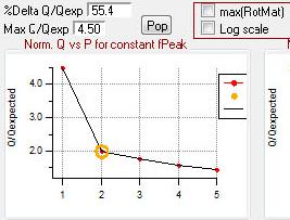
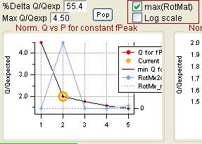
   • Exploration will run PMF for a range of number of factors and FPEAKs or SEEDs. This is the typical use for exploring a dataset and comparing many solutions.
   • Bootstrapping explores the uncertainty of one solution (i.e., one number of factors at one fpeak for one seed). This is usually a final step run only on the solution you have selected from the exploratory analysis.
4. Choose a range for number of factors.
   • When checking to make sure that everything runs properly, you may want to run just one case (Min p = 2, Max p = 2).
   • Recommended Practice: Run cases with 1 factor to have a context for the meaning of the 2-factor solution.
   • In the Bootstrapping mode, only the "min p" is read; the "max p" is ignored.
5. Choose FPEAK or SEED values
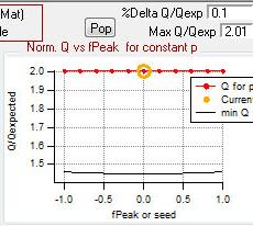
   • "FPEAK" is a tool used to explore rotations of the solutions of a given number of factors. Note that FPEAK does not explore all possible rotations of a solution. FPEAK = 0 does not apply any rotational forcing. Non-zero values of FPEAK create near-zero values in the factor profiles (mass spectra) or time series. More information about FPEAK can be found in the PMF Users Manual Part 1 (pp. 9,12,14,21) and Part 2 (p. 24), and in several papers by P. Paatero (see Other Resources).
     • A good first set of FPEAK values is -1.0 to +1.0 with a delta value of 0.1 or 0.2. For a full analysis, a wide enough range of FPEAKs to achieve Q/Qexp of at least 1% above the minimum value is recommended.
     • In Exploration mode when varying the fpeaks, the Seed is set in headers in the PMF_Execution...ipf file: constant DEFAULT_SEED = 0
     • In Bootstrapping mode, only the "min fpeak" is read; the "max fpeak" is ignored.
   • "SEED" is a tool used to choose different random starts (initial values) for the PMF algorithm. Using different seeds may lead to solutions in different local minima (Q/Qexp) in the solution space. One set of solutions may have more physical meaning than another, or multiple sets may make physical sense. It is impossible to test all start values, but testing many seeds may give an indication of local minima for your dataset. More information about seeds can be found in the PMF Users Manual Part 1 (p. 11) and Part 2 (p. 16).
     • Run seeds from 0 to your preferred maximum with a delta value of 1.
     • In Exploration mode when varying the Seed, the fpeak is set in the headers of the PMF_Execution...ipf file: constant DEFAULT_FPEAK = 0
       • Exploring Seeds with a non-zero fpeak should be done with caution, as the "push" of a magnitude of fpeak for one area of local minima may be different than the "push" of the same magnitude of fpeak for a different area of local minima.
     • In Bootstrapping mode, the Seed is set in headers in the PMF_Execution...ipf file: constant DEFAULT_SEED = 0
6. Select checkboxes
   • Run PMF in background Each execution of PMF (see Exploration Mode Summary) creates a black DOS window that pops up. If the box is not checked, this window "grabs the focus" and makes itself the top window. This makes it hard to use the computer for anything else. If the box is checked, the window will not grab focus, but Igor and your computer's CPU will be busy.

What the Software Does When You Press the Button...

Exploration Mode Summary

The software will execute PMF once for every combination of number of factors and FPEAK/seed. So if you run 1-5 factors and 5 FPEAKs, PMF will run 5x5=25 times. Each run starts a new black DOS window that will close when the run is completed. The duration of each run is printed in the history at the end of each run. In general, runs which solve for more factors and runs with FPEAK farther from 0 take longer. The code runs all of the FPEAKS or seeds for one number of factors, then advances to the next number of factors (e.g., run 1 factor with each of 5 FPEAK values, then 2 factors with each of 5 FPEAK values, etc.).

A little more detail

The software writes the files

C:\delete_log.bat    C:\runPMF.bat

and writes your DataMatrix and ErrorMatrix as MATRIX.DAT and STD_DEV.DAT, respectively to the folder with your PMF Executable. The software also writes a file to that folder called STD_DEV_PROP.DAT, which has the same number of points as the DataMatrix and in which every element is equal to the ModelError.

The software then enters a pair of nested loops in which the following steps occur:

• for each number of factors
  • for each FPEAK or SEED
    • use the file

 mypmft.ini

as a template to create the file

 imupmf.ini

which is used as the control file for PMF.

• In v2.03, the convergence criteria for completing the PMF calculations can be set proportional to Q/Qexp by changing headers in the PMF_Execution...ipf. The default is to use the convergence criteria in mypmft.ini.

 //Settings for PMF Iteration Convergence proportional to Qexp
 constant ITERATION_CHI2_PROP_QEXP = 0
 constant FIRST_ITER_LEVEL_PROP_CONST = 2e-6
 constant SECOND_ITER_LEVEL_PROP_CONST = 2e-6
 constant THIRD_ITER_LEVEL_PROP_CONST = 1e-6

You can read more about convergence criteria and large datasets in the PMF Users Manual Part 1 (pg. 10) (see Other Resources).

• Delete the old PMF2.LOG file by running delete_log.bat
• Execute PMF by running run_PMF.bat.
• Wait for PMF to complete its run.
• Load PMF output (including log file and factors)

At the completion of the loops, the software calculates some statistics from the output and then creates a panel to select data for viewing.

Bootstrapping (added in v2.02)

The bootstrapping mode is developed after the method described in the EPA PMF v3.0 Users Manual Sect. 6.4 (see Other Resources). The bootstrapping method is used to estimate the uncertainty in both the factor mass spectra and time series. This is achieved by running PMF on the full dataset once and then making a series of variations (the number is specified by the user when selecting the bootstrapping mode) in which a subset of the original rows (mass spectra) are randomly replaced by other rows from the original matrix and running PMF on each of these.

For each new PMF case ("bootstrapped case"), the resultant factors are compared to those from the original dataset and assigned as "matching" the original factor with which it has the highest correlation. Bootstrapped cases in which each bootstrapped factor was matched to exactly one of the original factors (i.e., there is a one-to-one mapping between original factors and those from the individual boot-strapped cases) are retained for calculation of the average mass spectrum and time series of bootstrapped factors. Plots of the original factors and the average bootstrap factors with 1-sigma variation bars are produced automatically.

EPA PMF Users Manual recommends doing 100 bootstrap runs for final results.

A little more detail

All output from the bootstrapping runs is saved in folder root:pmf_bootstrap:.

Row (mass spectrum) replacement is performed by using the StatsResample function in Igor to select rows for replacement. The row values are then sorted in increasing order as a convenience.

• The 2d wave RowsToBeReplaced records the rows to be used in each bootstrapped case. Each column represents one bootstrap case. Each column lists the rows of the original matrix included in that bootstrapped case.
• The 2d wave ReplacementHistogram counts the number of times that each original matrix row was used in a bootstrap case. Each column represents one bootstrap case. Summing the rows of this matrix gives the total number of times that each original matrix row was was used in the bootstrapping cases.

The assignment of bootstrapped factors to the factors from the original case is made by Pearson R correlation. Factors are assigned only on the basis of mass spectral comparison, and each factor is assigned to one of the original factors.

• Note that this is different than in EPA PMF. Our code does not have a criterion for the lowest allowable correlation between bootstrapped and original factors. In EPA PMF, factors that fall below this limit are "unmapped"; no factors are "unmapped" in our code.
• Note that if the original case has factors that are very similar to each other, the assignment of the bootstrapped factors may be incorrect or ambiguous. No current work has been done to give guidance as to what "very similar" means. No sanity checks are made in the code for this type of situation.
• The 3d wave FactorProfile_Rval stores the correlation between the boostrapped and original factors. Rows represent the factors from the original case, columns represent the factors from the bootrapped cases, and layers represent each bootstrapped case.
• The 2d wave FactorProfileSort contains the number of the original factor to which each boostrapped factor (row) has been matched in the bootstrapped case (column). Columns which contain (e.g., in a case with three factors) "0, 1, 2" have factors which were uniquely matched to the columns in the original case; these will be included in the averages of mapped factors. Columns which contain duplicate entries (e.g., "0, 1, 0") have multiple factors that were matched to the same original factor; these cases will not be included in the averages of the mapped factors.

Note that the criteria for including bootstrapped cases in calculations of the average bootstrapped factors is different in our code than in EPA PMF. Bootstrapped cases in which two or more factors are mapped to the same original factor are not included in the averages in our code. In these instances, the whole bootstrapping case is rejected before calculating averages. In EPA PMF, all bootstrapped factors mapped to the same original factor are included in the average.

Important: At the present time (v. 2.02) the plots produced by the bootstrapping code expect to find the waves noNaNs_amus (for plotting profiles) and noNaNs_t_series (for plotting time series). If these are not the names of your waves that describe the columns and rows, respectively) of the input matrix, you should duplicate your row and column description waves to have these names.

Running Two Simultaneous Analyses on Dual-Processor Computers

You can run two PMF analyses (in two separate experiments) on the same computer simultaneously if you have dual processors. Each analysis will run at the same speed as on a single-processor computer (or when one analysis is run on the dual processor computer). The PMF executable is not "multi-processor aware," meaning that it can not utilize both processors simultaneously for one PMF run.

To run two simultaneous analyses with the PET, you'll need two directories on your computer with the PMF .exe, .key, and mypfmt.ini files. The directory names must end in "1" and "2," respectively. For example, you could have

C:\PMF\PMF Executable1

pmf2wtst.exe

pmf2key.key

mypmft.ini

C:\PMF\PMF Executable2

pmf2wtst.exe

pmf2key.key

mypmft.ini

Each experiment running PMF must use a separate Executable directory. While a PMF analysis associated with a PMF Executable directory is running, a file called "PMFrunning.txt" exists in that directory. If you try to run your second PMF analysis using the same Executable directory, the PET will give you an error. You can choose a different Executable directory and press the button to start the analysis.

View PMF Analysis Results *Step 2*

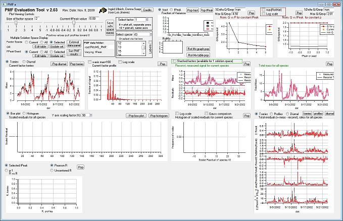
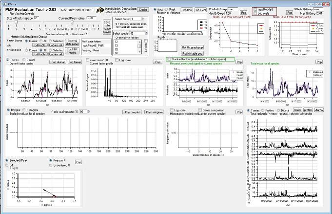
This is a clickable picture of the main PMF panel. Clicking on a region will take you down the page to more information on the options possible for that control or graph.

<imagemap> Image:PMF_Evaluation_Tool.jpg|1000px|alt=PMF_Evaluation_Tool rect 3 24 403 120 Factor Space and Fpeak Slider rect 408 53 443 116 Save Solution Space Waves rect 447 41 594 93 Select Factor rect 447 96 594 203 Select Species rect 7 117 251 204 Select Multiple Factors or Fpeak/Seed rect 608 3 837 122 Mass Fraction/Variance rect 608 120 840 204 RotMx rect 840 2 1077 208 Q versus Number of Factors rect 1076 3 1312 202 Q versus fpeak/seed rect 3 210 330 413 Time Series rect 333 209 657 412 Profiles (usually Mass Spectra) rect 990 215 1312 408 Total Reconstruction rect 992 415 1312 820 Total Residuals rect 662 204 987 414 Current Species Reconstruction and Residual rect 5 413 661 618 All Species Scaled Residuals rect 661 414 989 619 Current Species Scaled Residuals rect 3 620 331 819 "RR" Plot desc bottom-left </imagemap>

Controls

Factor Space and Fpeak Slider

Save Solution Space Waves

Select Factor

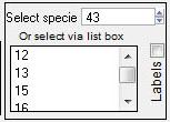
Select species

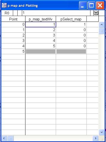
Select Multiple Factors or Fpeak/Seed

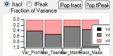
Mass Fraction

Mass Fraction/Variance

RotMx

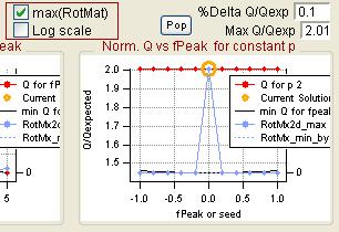
Q Plots

Q versus Number of Factors

Q versus fpeak/seed

Factor Graphs

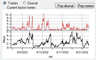
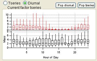
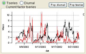
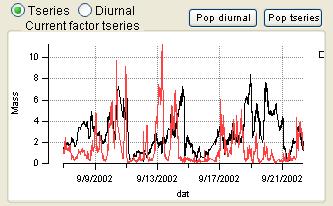
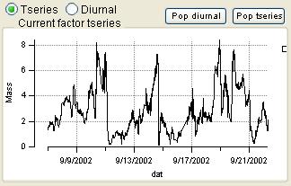
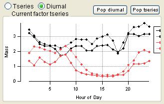
Time Series

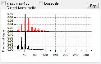
Profiles (usually Mass Spectra)

Reconstruction and Residuals

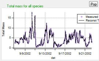
Total Reconstruction

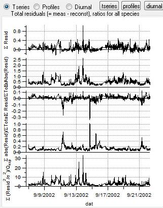
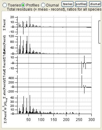
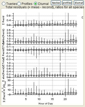
Total Residuals

Current Species Reconstruction and Residual

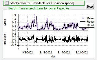
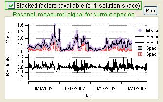
Scaled Residuals

All Species Scaled Residuals

Current Species Scaled Residuals

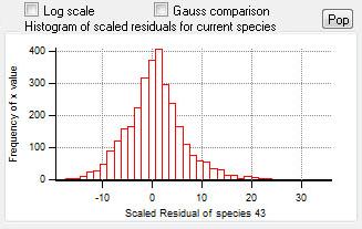
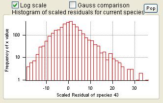
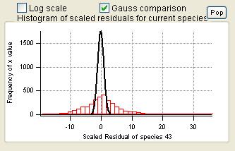
"RR" plot

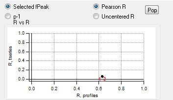
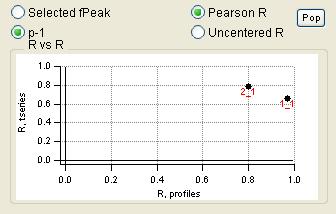
Compare PMF Results with External Factors *Step 3*

Caution: This part of the code is a bit fussy! Please contact Ingrid if you have tried the tips here and have trouble getting this panel to work.

Setting up the External Data

1. Check that the strings "NaNsList_amus" and "NaNsList_t_series" (these were created when you deleted NaNs from your original matrix) are in the datafolder where your PMF output is being saved. If they're not already there, you'll need to find them and copy them to this location. They need to be created as global strings (e.g., string/G NaNsList_amus = otherWaveLocation).
2. You'll need separate folders (in root: ; they cannot be in a lower directory) for mass spectra and time series you want to use for comparison to the factors.
   • The tricky part of using this panel is setting up your mass spectra and time series correctly.
   • Each wave must have either the same number of points as in the corresponding dimension of your noNaNs_ data matrix or the same number of points as in the corresponding dimension of your original matrix.
     • For example, if your original matrix is 3246 rows and 300 columns and your noNaNs_ matrix is 3200 rows and 268 columns, your "external" mass spectra can have 300 or 268 points; "external" time series can have 3246 or 3200 points.
   • For mass spectral comparisons, download "full" spectra (usually 300 points) from the AMS Spectral Database instead of using the shortened ones provided in the 9th Users Meeting template. You should inspect the length of all waves from the Database to make sure that every one has the correct number of points for your work.
3. IMPORTANT NOTE 1: The reason for the restriction on the number of points in "external" comparison waves is the following: After you select the datafolders for the external mass spectra and time series, the code makes a folder inside each of these folders called "noNaNs". Each wave in the external datafolder is copied to the new directory. Then the code checks whether the waves have the same number of points as the same dimension in the matrix used to run PMF; if so, no change is made to the wave. If not, the code _assumes_ that the wave has the dimension of the original matrix (which it doesn't know about) and therefore uses the string "NaNsList_amus" or "NaNsList_t_series" to delete the rows that it believes were NaN in the original dataset. (It's ok if these waves still have NaNs (e.g., missing points in data from another instrument when the AMS data was good); only the points where both the factor and external waves have valid data are included in the correlation calculation.)
4. IMPORTANT NOTE 2: The mass spectra in the AMS Spectral Database have m/z = point number, meaning that point 0 = m/z 0. This is not usually the way that AMS matrices are saved from James' software or from Squirrel, so you probably need to delete 1 point from the beginning of each spectrum that you use from the Database.
5. IMPORTANT NOTE 3: Because of some internal coding restrictions, time series waves for comparison cannot include the string series in their name; such waves will not be created in the noNaNs folder.

Choosing the Folders with External Data

1. The first time you want to calculate factors you can do so by pressing the "External Data Panel" button on the main panel or by choosing from the PMF pulldown menu "Compare PMF results with External Factors *Step 3*".
   • Note that after you have accessed the "External Data Locations" panel, pressing the "External Data Panel" button on the main panel will not bring you back to the selection panel again. To choose different folders or force recalculations you must access the selection panel from the PMF pulldown menu.
2. Select your external data folders.
   • Other choices from the pulldown menus include
     • "No external data of this type": The PET will not attempt to calculate correlations between factors and external data of this type.
     • "Update List": If after calculating factor correlations you wish to add new external waves of this type, choose this option to add the correlations for the new waves do your existing list of correlations.
3. Press the button to proceed.

What the PET Does (and how to fix things if something goes wrong)

1. In each external data folder, a folder called "noNaNs" is created as described in the IMPORTANT Note 1 above (item 3 of Setting Up the External Data).
2. Each of these new waves is compared to every factor wave. (This can take a while if you have a lot of waves for comparison.)
   • If the factor and external waves have different lengths, the function aborts and tells you that the comparison function was called with waves of different lengths. Unfortunately, it doesn't give helpful information about which wave had the wrong length (we'll try to look into that and improve that error message).
     • If this happens, you should look in the "noNaNs" folder in the appropriate external data folder and check whether all of the waves have the correct length. Waves with incorrect numbers of points in this folder may be the result of incorrect wave lengths in the "external data" folder. Try to fix all of the problem waves and then run the function for calculating the scatter comparison again by choosing step 3 from the PMF pull-down menu. Recall that this is the only way to force recalculation of the comparison of the factors!
       • If forcing recalculation didn't fix the problem, delete the "noNaNs" folder in the appropriate external data folder and then recalculate again.
3. The correlation values between the factor waves and the external data waves are stored in waves in the folder with PMF output called
   • • "RcorrMx4d_Profiles" and "RcorrMx4d_Tseries" (with Pearson R)
     • "RcorrMx4d_Profiles_pear_mzGrt44" (with Pearson R, only for m/z > 44)
   • It is also possible use the function scat_calc_RCorrMx4d_UC() to calculate
     • "RcorrMx4d_Profiles_UC" and "RcorrMx4d_Tseries_UC" (with the Uncentered Correlation, as reported in [ Ulbrich et al., ACP, 2009]
4. When the calculation is complete, the Scatter Panel is created.

Other Potential Problems and Solutions

• Pulldown menus don't have lists. Each "noNaNs" folder should also contain a text wave called "TseriesWvsNms" for time series or "FactorWvsNms" for profiles. This wave is used for the pulldown menus in the panel. If this wave is missing, the pulldown menus may not work. There should also be a string of wave names in the folder called "TseriesWvsNmsList" or "FactorWvsNmsList"; if so, you can create the text wave by gen_list2txtWv(listStr, wvNm).

Some Other Notes

• Order of the factors. Factors are numbered 1 to N and match the factors in the main panel, counting from the bottom of the factor plots.
• Colors. Factor 1 is black, Factor 2 is red, Factor 3 is green, Factor 4 is blue, etc. Factors in this panel have the same color as they did in the main panel. In the overlay plots, the factor is its usual color and the external species is orange.
• Size of Factor Space and Current Fpeak value sliders. The sliders in this panel and in the main panel control both panels simultaneously. Graph updates are slower with both panels. Be patient and don't click on anything until everything has updated.

More Features

• Assign Groups to External Data. This feature allows you to reorder the external data waves and assign them to groups. Groups then define the colors used in the R bar plots in the panel and in the Comprehensive External Data Correlation Plot (below).
• Comprehensive External Data Correlation Plot. This plot display the "R vs External Factor" plots for all factors at once.

PMF Evaluation Tool Software

Version	Date	Release Notes	Error Prep ipf files	3 PET ipf files		PET Template		mypmft.ini
2.03A	21 Jan 2010	Release Notes v2.03A	pmf_ErrPrep_AMS_v2_3A.ipf	PMF_Execution_v2_03A.ipf PMF_ViewResults_v2_03A.ipf PMF_scatter_v2_03A.ipf	or	Igor PMF Template v2.03A	and	mypmft.ini for use with v2.03 and higher
2.03	9 Nov 2009	Release Notes v2.03	pmf_ErrPrep_Q-AMS_OneIonEquiv_v2.3.ipf pmf_ErrPrep_ToF-AMS_OneIonEquiv_v2.3.ipf pmf_ErrPrep_AMS_v2_3.ipf	PMF_Execution_v2_03.ipf PMF_ViewResults_v2_03.ipf PMF_scatter_v2_03.ipf	or	Igor PMF Template v2.03
2.02	18 May 2009	Release Notes v2.02		PMF_Execution_v2_02.ipf PMF_ViewResults_v2_02.ipf PMF_scatter_v2_02.ipf	or	Igor PMF Template v2.02	and	mypmft.ini for use with v2.0 and v2.02
2.0	29 Aug 2008	Release Notes v2.0		PMF_Execution_v2_00_RC1.ipf PMF_ViewResults_v2_0_RC3.ipf PMF_scatter_v2_0.ipf	or	Igor PMF Template v2.0

BareBones Starter Kit

Download the BareBones_PMF_Starter_Kit.zip described for initial installation of PMF on a computer.

Other Resources

• FTP sites with PMF code, documentation
  • P. Paatero's list of PMF url's (working on 13 May 2009)
    • The PMF order form (PMFORDER.pdf) can be found from Paatero's site in this zip file
  • P. Hopke's mirror of Paatero's site (working on 12 May 2009)
• Ingrid's presentation of the PET at the 9th AMS Users Meeting in three parts (1. Overview and PMF Execution; 2. Viewing PMF Results; 3. Using the Scatter Plot Panel)
  • The tutorial data used with that presentation
• The AMS PMF Resources page, with releases of the PET and some sample data.
• EPA PMF and its documentation

Some PMF Method Papers

• Paatero, P., and Tapper, U.: Analysis of different modes of factor analysis as least squares fit problems, Chemom. Intell. Lab. Syst., 18, 183-194, 1993. Abstract

• Paatero, P., and Tapper, U.: Positive Matrix Factorization: a non-negative factor model with optimal utilization of error estimates of data values, Environmetrics, 5, 111-126, 1994. Abstract

• Paatero, P.: Least squares formulation of robust non-negative factor analysis, Chemom. Intell. Lab. Syst., 37, 23-35, 1997. Abstract

• Paatero, P., Hopke, P. K., Song, X. H., and Ramadan, Z.: Understanding and controlling rotations in factor analytic models, Chemom. Intell. Lab. Syst., 60, 253-264, 2002. Abstract

• Paatero, P., and Hopke, P. K.: Discarding or downweighting high-noise variables in factor analytic models, Anal. Chim. Acta, 490, 277-289, 10.1016/s0003-2670(02)01643-4, 2003. Abstract

• Paatero, P., Hopke, P. K., Begum, B. A., and Biswas, S. K.: A graphical diagnostic method for assessing the rotation in factor analytical models of atmospheric pollution, Atmos. Environ., 39, 193-201, 10.1016/j.atmosenv.2004.08.018, 2005. Abstract

• Paatero, P., and Hopke, P. K.: Rotational Tools for Factor Analytic Models, J. Chemom., 23, 91-100, 10.1002/cem.1197, 2009. Abstract