Field Data Analysis Guide
Contents
- 1 Introduction
- 2 A Message for Contributors
- 3 ToF-AMS Process Flowchart
- 4 Process Calibrations
- 5 Process Unit Resolution Data
- 5.1 Load data into Squirrel, Inspect Diagnostics
- 5.2 Perform m/z Calibration
- 5.3 Perform Baseline Subtraction
- 5.4 Pre-process data
- 5.5 Perform air beam correction
- 5.6 Make campaign specific adjustments to fragmentation table
- 5.7 Make average mass spectra plots of filter periods to double check fragmentation table modifications
- 5.8 Generate time series and average spectra of unit-resolution data
- 5.9 Choose preliminary CE from observed composition and accumulated AMS experience
- 5.10 Look a MS and size distributions of very large outliers, blacklist if appropriate
- 5.11 Work up comparisons of total mass and volume with other instruments
- 5.12 Make size distributions for a handful of periods with good signal
- 5.13 Work up comparisons of size distributions for those same periods with other instruments
- 5.14 Reevaluate CE choice based on intercomparisons
- 5.15 Start looking at the scientific questions of interest
- 5.16 Mission Diagnostics Plot
- 6 Determining Precision Directly from Field Data
- 7 Reporting your data
Introduction
The ToF-AMS Field Data Analysis Guide is dedicated to the analysis of complex ToF-AMS field data sets and is intended to establish standard practices in this area on a community-wide basis. It is assumed that users will have some familiarity with Igor and the community based AMS analysis tool, Squirrel. Preliminary AMS data can be generated while a project is underway without worrying about some details; this guide is intended for identifying all post-project analysis steps involved in generating final data.
A Message for Contributors
We want to encourage active participation by all ToF-AMS users in the evolution of the information contained within this wiki and welcome the addition of content that is beneficial to the community as a whole. However, please DO NOT delete any content from this page!! Significant time, effort, and deliberation has gone into the information contained in this page. Rather than deleting content, please feel free to voice your concerns by posting a comment to the discussion page where others can contribute (please be sure to include a topic to be referenced in responses).
ToF-AMS Process Flowchart

Process Calibrations
Determine Flow Rate Calibration
- Basic Principle: AMS flow rate is used to convert MS signal intensity to units of mass concentration. Flow rate is derived from lens pressure (analog input #3) and converted using a conversion factor. Post-correction of flow rate MUST be performed if there is:
- any deviation between the derived and calibrated flow rates;
- errors in the logged flow rate value;
- electronic noise, or;
- drift in the zero of the baratron.
- In the absence of errors, flow correction is made by multiplying the logged flow rate by the ratio of derived to calibrated flow rates. To correct for errors, the calibrated flow rate must be used.
- NOTE: Save backup of flow rate wave (located in root:diagnostics) and construct new, corrected flow rate wave in Squirrel data analysis experiment. This new wave MUST be named “flowrate”.
- Data Recording: A flow calibration MUST be performed at least once in the field using a Gilibrator.
- How Calculated:
Flow ratecorrected = flow ratederived x (flow ratecalibrated/flow ratederived)
- How Applied: Flow rate is used in the calculation of Squirrel component mass concentrations:
- Squirrel Code:
- Function: SQ_MS_Concentration
- ugfac=ug_op?((aw/Navo)*1e12/(ioneff_wave[p1]*flowrate[p1]*rie*ce)):(1)
- Squirrel Code:
- Recommendations:
- Begin Mission Diagnostics Plot by adding the original and modified flow rate data.
- Additional Resource: See Q-AMS manual for more information on correcting flow rate.
Determine Time Line of Single Ion Values
- Basic Principle: The single ion (SI) value is used to convert MS signal intensity to units of mass conc. SI values logged by the data acquisition software may not be the true values. Unlike threshold values, single ion values can (and in many cases must) be post-corrected by applying a new set of values prior to pre-processing the data.
- Data recording: It is recommended that the threshold analysis be performed daily to have adequate data for timeline of SI values.
- How Modified: Single ion values should be obtained in the field using the threshold analysis window within the data acquisition software. If post-correction of the single ion values is required, this change can be made by clicking the Modify SI button in the “Optional Checks & Advanced Features” (HDF Index tab).
- NOTE: Any change in single ion values MUST be made prior to pre-processing.
- How Applied: SI value is applied in Squirrel to convert bit*ns to ions/s (Hz)
- Squirrel code:
- Function: sq_Hz(index_pos,datawav)
- wave ion_wave=root:diagnostics:ionSingleStr_logged
- datawav*=(1/ion_wave[series_index[index_pos[p]]]) * ToFPulserInHz[series_index[index_pos[p]]]
- Squirrel code:
- Recommendations:
- Add original and modified SI time series to the MDP.
Process all IE/RIE_NH4 Calibrations
- Basic Principle: The ionization efficiency (IE) calibration determines the ionization efficiency of ammonium nitrate. Quantification of all non-refractory AMS components are based on the linearity of this IE (i.e., the IE for all species can be related to the measured IE of a single species, in our case NO3).
- Data Recording: It is recommended that all IE calibrations be recorded periodically during sampling with the data acquisition software running in GenAlt Mode.
- How Derived: ToF-AMS IE calibrations are typically performed in the field using BFSP mode. Software is available to analyze these IE calibrations at the ToF-AMS Resource Page. A tutorial regarding BFSP IE calibrations is also available here. This software should be used to determine IENO3 and RIE_NH4 values for each field IE calibration. RIE_NH4 should be double checked using MS mode data.
- How Applied: Calibrated ion efficiency is applied in the calculation of Squirrel component mass concentrations.
- NOTE: Airbeam correction also influences the IE and will be discussed later (add link).
- Recommendations:
- Add IE calibration data (IE, AB, and flow rate) to the MDP.
- Additional Resource: See Q-AMS manual for more information on IE calibrations.
Evaluate SI, IE, RIE_NH4 to use, based on SI, IE, AB, flow, and IE/AB for the whole campaign
- Basic Principle: Based on results of threshold analyses and IE calibrations performed during the campaign select single ion (SI), ionization efficiency (IE), and ammonium relative ionization efficiency (RIE_NH4) values for the entire campaign.
- How Derived:
- Ideally, these values are simply the averages calculated from all evaluations (i.e., threshold analyses and IE calibrations) performed during the campaign.
- However, it is likely that the time lines of these values will need custom corrections. This is particularly true of the time series of the time line of the IE value.
- A critical parameter used to finalize the IE time series is the (IE/AB)Correction value.
- How Applied: After deciding on correct values:
- SI values can be modified using the Modify SI button in the “Optional Checks & Advanced Features” (found in the "HDF Index" tab)
- IE values:
- if no correction needed, the average IE will be used during the AB correction.
- When doing AB correction, “ioneff” is written to single constant value.
- If autoset is not used when performing an airbeam correction, then “ioneff_logged” is never used.
- If correction needed, see Discussion
- for Squirrel versions earlier than 1.38, use a post-correction function
- For Squirrel versions 1.38 and later, use “ioneff_to_AB_ratio_rel” and “user_corr_fac”.
- RIE_NH4 value should be used to modify the batch table.
- Recommendation:
- Add final SI to the MDP along with logged and user corrected IE values.
- NOTE: When modifying SI and IE values, “*_logged” waves should never be changed as these changes will be overwritten whenever you perform a squirrel diagnostics.
IE/AB Correction
- Basic Principle: The ToF-AMS ionization efficiency (IE) measures the sensitivity of the instrument to a measured quantity of a specific compound, typically NH4NO3, during instrument calibration. Throughout sampling, this sensitivity is reflected by changes in the instrument air beam (AB). In most cases, changes in sensitivity are observed in the AB and will be accounted for when performing an AB correction. However, there are instances where this may not the case and a custom correction is needed. The parameter that can be used to evaluate the need for a custom correction is the IE/AB ratio ((IE/AB)calibration) obtained from each IE calibration. If the (IE/AB)calibration for calibrations performed throughout the sampling period do not change significantly an IE/AB correction is not needed. If these values are not constant, a correction is required.
- In Squirrel versions 1.38 and greater, an IE/AB specific correction wave “ioneff_to_ab_rel_ratio” has been implemented to aid the user. However, in Squirrel versions prior to 1.38, this wave must be created and the correction must be implemented manually.
Application of IE/AB Correction
- Basic Principle: The intended use of the “ioneff_to_ab_rel_ratio” wave is to account for circumstances where the (IE/AB)calibration changes over time. In Squirrel versions 1.38 and higher, this wave is present by default with values set to 1. For earlier Squirrel versions, this wave will need to be created. In either case, “ioneff_to_ab_rel_ratio” MUST be modified to account for changes in (IE/AB)calibration values.
- How Calculated: The values in the “ioneff_to_ab_rel_ratio” wave can be calculated by first establishing a correct, initial IE/AB value (IE/AB)t=0 (typically from an early IE calibration). The value of the required correction factor at each subsequent timestep, i, is then calculated by dividing (IE/AB)t=0 by the IE/AB ratio at this time (IE/AB)i:
ioneff_to_ab_rel_ratio[i] = (IE/AB)[i] / (IE/AB)t=0
- A time series of (IE/AB)[i] can be constructed by interpolating linearly between the (IE/AB)calibration values from each IE calibration.
- How Applied:
- In Squirrel versions 1.38 and above “ioneff_to_ab_rel_ratio” is automatically applied to adjust the species mass concentrations through the SQ_MS_Concentration function.
- In Squirrel versions prior to 1.38 a post-correction function should be used to apply a corrected IE time series (that has had the IE/AB correction factor applied), through the following convention:
ioneff_corr = ioneff * ioneff_to_ab_rel_ratio
- Recommendations:
- Add the IE/AB corrections wave, if created, to the MDP.
Process size calibrations
- Basic Principle: The parameters contained in the data acquisition software to describe particle time of flight may not be correct and need to be re-evaluated using the polystyrene latex (PSL) particle size calibrations performed in the field.
- Data Recording: It is recommended that size calibrations be performed during the field deployment using 100, 300, 500 , 700, and 900 nm PSL particles. Sizes at or below 100 nm can be obtained with the classifier after it is calibrated at 100 nm.
- How Derived: The size calibration is calculated by fitting a plot of particle size (Dva,PSL) vs. average particle velocity (Vpart, in m/s) using the following fit function:
Vpart = f(Dva,PSL) = Vl + (Vg - Vl) / (1 + (Dva,PSL/D*) ^ b)
- Dva = vacuum aerodynamic diameter;
- Vl = lens velocity, and;
- Vg = gas velocity
- NOTES:
- 1. The time component of the Vpart calculation is obtained using the left (leading) edge of the ToF distribution. For choppers with a duty cycle >=2% and for calibrations with PSL, one-half of the chopper width should be added to the edge time. One-half chopper width is calculated as (0.5*duty cycle)/chopper frequency (e.g., 71.4 us for a 2% chopper at 140 Hz).
- 2. The distance component of the Vpart calculation is the length of particle flight chamber. For the AMS, these are:
- 0.293 m (short chamber);
- 0.39 m (long chamber).
- 2. The distance component of the Vpart calculation is the length of particle flight chamber. For the AMS, these are:
- 3. To convert nominal diameter to vacuum aerodynamic diameter:
Dva = dp * p * S
- Dp = nominal diameter
- S = Jayne shape factor (S = 1 for PSL), and
- p = density (p = 1.05 for PSL)
- 4. Other fit functions can be used as long as that fit interpolates the data points.
- 5. For the default fit equation, initial guesses for each coefficient are as follows:
- Vl = (10-25)
- Vg = (450-650)
- D* = 20
- b = 0.50
- 5. For the default fit equation, initial guesses for each coefficient are as follows:
- In some cases, the lens velocity resulting from the fit can be negative. Under these circumstances, either Vg or Vl should be held constant within the range of values suggested above. It should be noted, however, that constaining Vg within the suggested range can still result in a negative Vl.
- 6. Periods with different flowrates (changes in orifice, clogging) need to have different calibrations.
- How Applied: Parameters obtained by fit will be used to recalculate aerodynamic diameters when performing corrections in Squirrel.
Process Unit Resolution Data
Load data into Squirrel, Inspect Diagnostics
NOTE: Prior to loading data in squirrel, it is strongly recommended that the user review the General and Technical FAQs listed on the Squirrel main page as well as the several tutorials that are available on the Squirrel Help page
Squirrel requires AMS data to be saved in .HDF format. Under normal operating conditions, data is saved automatically by the data acquisition software in both .ITX and .HDF format. If .HDF files were not saved during sampling, the user can use the HieDI file converter to convert the .ITX files.
To load .HDF data into Squirrel:
- Press “Get Index” button;
- Browse to folder containing .HDF data files.
After indexing the .HDF data, Squirrel creates a diagnostics plot that can be used to diagnose the data set.
Implement Corrected Flow Rate and Single Ion Values, if any
- Basic Principle: As discussed previously, incorrect flow rate and single ion values must be corrected prior to Squirrel data pre-processing because these values are used to convert AMS signal intensity to mass concentration during this step. Once data has been pre-processed, the single ion values are “set” and correcting any errors requires repeating data pre-processing. Therefore, it is strongly suggested that the user devote significant effort to ensure that the single ion values are correct and final before moving on. If no changes are made, pre-processing will use the flow rate and single ion values that were captured by the data acquisition software. These values are shown in the Squirrel diagnostics plot, which can be used as a reference.
- Data Recording: N/A
- How Derived: N/A
- How Applied: Recommended ways of modifying the flow rate and single ion values prior to data pre-processing were presented previously. See previous flow rate and single ion value discussions for more details.
- Recommendations:
- Notes:
- Generally, it is recommended that the AMS flow calibration be expressed in terms of mass rather than volumetric flow.
- Reported mass concentrations are dependent on the calibrated instrument flow rate. Therefore, the conditions under which the instrument flow rate was calibrated in the field should be reported in all manuscripts (e.g., at STP or ambient and, if ambient, under what conditions).
Discard Bad Runs (from notebook, large noise, or low sampling time)
Bad runs can sometimes produce huge concentrations that are not real. Often new users forget to remove those runs, and their averages, scatter plots, etc. get hugely distorted. Reasons for bad runs include the inlet valve that was closed during part or all the run, cell phone noise, some electronic switch (e.g. heater bias from manual to computer) being changed during the run, and many others.
To discard runs, just type the run numbers in the appropriate box in Squirrel and hit "discard." Try to be thorough, and remove all runs identified as bad in the notebook. If you are not sure whether a run is bad, look at its mass spectra and size distributions, and it generally becomes clear whether the data is good or whether it has some major problems.
Perform m/z Calibration
- Basic Principle: Under normal operating conditions, the user calibrates the instrument via the data acquisition software during instrument start-up. Afterwards, the ToF-AMS data acquisition software automatically calibrates m/z during autosave operation to account for drift in the calibration over time. Squirrel m/z calibration SHOULD be performed as a first step in ToF-AMS data analysis to ensure correct assignment of peak location in order to convert the raw data to stick format. The m/z calibration has to be performed prior to data pre-processing in order for the Squirrel fitting parameter values to be available as an option during pre-processing.
- Data Recording: Initial m/z calibrations are required after restarting EITHER the instrument OR the acquisition software.
- How Derived: N/A
- How Applied: The m/z fitting procedure is initiated by clicking the “Check m/z calibration” button and then the “Begin mz fitting” button after the SQ_MzCalibration_Panel window appears.
- Recommendations:
- For most fragments, use closed spectrum for m/z fitting (exceptions are air peaks (N+, O+, and Ar) for which open spectra can be used);
- C+, O+, and the Tungsten series have been found to be problematic for some data sets. In this case, these fragments should be removed when performing the m/z calibration;
- It is recommended that the user have at least one peak greater than m/z 90;
- At present, the calibration as performed cannot reliably be extrapolated to masses larger than m/z 200. This may be fixed in future Squirrel releases. As a result, if the exclusive focus of the analysis is large mass fragments, the user should remove all low mass fragments from the mass table prior to performing the mass calibration.

- 1. Using the inset table, the user can modify the fragments used in the m/z calibration prior to beginning m/z fitting. To remove a fragment from the fitting procedure, place a zero in the corresponding cell in the SpecType column. The table can be reset to default values by clicking the “Revert to Default” button. Peaks from the closed spectra are typically better with the exception of the air peaks, for which open spectra can be used.
- 2. After selecting the fragments to include in the fitting procedure, the procedure is started by clicking “Begin mz fitting”.
- 3. The accuracy of the m/z calibration and mass calibration for each run are displayed during m/z fitting. The accuracy parameter evaluates the “goodness of fit” of the Squirrel calibration relative to that of the acquisition program.
- 4. These plots display the results of m/z fitting from each run. The raw data (black dots) and the Squirrel fit (red line) are plotted along with the designated peak center determined from the data acquisition (black vertical line) and Squirrel (yellow vertical line) m/z calibrations.
- 5. The overall goodness of the Squirrel m/z calibration, relative to the calibration from the data acquisition program, is reported (ratios (data acquisition/Squirrel) for intercept, slope, and power). Deviation from unity represents a “bad” fit by the Squirrel m/z calibration.
- 6. “Bad” fits can be “filtered” after the m/z fitting procedure, if needed. The threshold criteria for filtering is the deviation of the ratios found in (4) from unity. The value of this threshold is at the discretion of the user as is the method used to fill in the bad fit value.
Perform Baseline Subtraction
- Basic Principle: ToF-AMS mass concentrations are derived from the difference spectra. Both raw open and closed spectra can have a significant non-zero baseline that is transferred to the raw difference spectrum as well. The “check baseline” routine allows the user to examine and make corrections to the baseline of the difference spectrum. This correction ensures that any baseline contribution to the stick value for each m/z fragment is removed prior to calculating the difference stick spectra.
- Data Recording: N/A
- How Derived: N/A
- How Applied: The check baseline procedure is started by clicking the “Check baseline” button, which will open the SQ_Baseline_Panel.
- Recommendations:
- Use mass defect wave as peak center and remove additional regions from stick complement (“Advanced Options” tab).
- Is there an objective way to say whether the baseline correction is good enough? (numerical estimate of corrected vs uncorrected)
Pre-process data
Perform air beam correction
- Basic Principle: As discussed above, the single ion strength (SI) and ionization efficiency (IE) is a fundamental quantities that need to be known in order report AMS mass concentrations. While it is not possible to continuously measure the SI and IE throughout the course of a sampling period, the air beam (AB) provides an indirect measure because of it's dependence on both. For this reason, it is important to note the AB as well as the IE when performing calibrations.
- The AB correction is used to account for changes in SI and/or IE throughout the course of sampling relative to a designated reference period. The AB correction factor (rer. corr_fact in Squirrel) compensates for changes in the AB over time by adjusting AMS mass concentrations as follows:
component conc.[i,ABcorrected] = component[i] * Corr_Fact
- The AB correction factor is calculated for each run in the sampling period as the ratio of the AB at the reference period to that measured at each step, i. Typically, reference periods are chosen immediately FOLLOWING an IE calibration (where the precise IE and its corresponding AB are well known).
- If the IE/AB ratio does not remain constant throughout the sampling period, the AB correction will NOT produce the correct answers. In addition to the AB correction, a seperate correction is required in this case (see this wiki, section 1.4.1).
- How Calculated:
Corr_Fact = AB[reference]/AB[i]
- Squirrel code:
- Function: SQ_MS_Airbeam()
- corr_fact=(j==detector_num[p])?(airbeamCorrToFTypeValue[1][j]/airbeam[p]):(corr_fact[p])
- Function: SQ_MS_Airbeam()
- Squirrel code:
- How Applied:
component conc.[i,ABcorrected] = component[i] * Corr_Fact
- Squirrel Code:
- Function: SQ_MS_Concentration()
- ugfac_wav_tmp*=corr_fact[p]
- Function: SQ_MS_Concentration()
- Squirrel Code:
- Performing AB correction in Squirrel: The AB correction can be found under the Corrections:Airbeam tab. Two options are available in Squirrel when calculating the AB correction: auto-set and non-auto-set.
- Active auto-set
- When the auto-set option is active, the reference period is selected by the user with the Squirrel marquee function (ref. Squirrel tutorials). Upon selecting an AB reference period, that range is automatically entered into the squirrel AB corrections panel and average values for the MS AB, IE, and flow rate from that range are calculated when performing the AB correction. It is important to use average values from the data set immediately following IE calibration instead of values from that calibration for consistency with data (e.g., the pressure in the inlet during calibration may be different from that observed during sampling which will cause the IE calibration to have a different AB value).
- Inactive auto-set
- If the auto-set option is not active, the MS AB, IE, and flow rate values from the reference period MUST be manually entered by the user (for the high resolution ToF-AMS, values for BOTH V and W modes must be entered paying special attention to the ToF/ion type).
- Recommendations:
- Add corr_fact and corr_fact_flow to the MDP.
- NOTE: It is IMPORTANT to note that, when the AB correction is perfomed, the IE value from the reference period REPLACES reference IE (wave name = ioneff) values in the Squirrel experiment if they exist. Therefore, if any custom modifications have been made to the IE time series prior to performing the AB correction, the user MUST reapply these modifications via a post correction function (add link to future section in this wiki).
Correct for Flow
- Basic Principle: The objective of the AB correction is to compensate for all changes in instrument sensitivity relative to the reference time period. While the majority of these AB changes can be attributed to changes in the IE and/or SI, the AB can also change with changes in flow rate. If the AB correction is applied before removing the flow rate changes errors are introduced into the data. Removing flow rate changes from the AB correction is accomplished by applying the "Correct AB for flowrate" option within the Corrections:Airbeam panel. (add screen shot of the flow rate box in the Squirrel panel).
- NOTE: The flow rate is ALWAYS applied to calculate mass concentrations regardless of whether this correction is applied.
- How Calculated:
Corr_fact_flow = (Flowrate[i] + Flowrate offset))/(Flowrate[reference] + Flowrate offset)
- Squirrel Code:
- Function: SQ_MS_Airbeam()
- If no smoothed flowrate:
- corr_fact_flow=(flowrate+airbeam_ref_flowOffset_sv)/(airbeam_ref_flow_sv+airbeam_ref_flowOffset_sv)
- If smoothed flowrate:
- corr_fact_flow=(flowrate_smoothed+airbeam_ref_flowOffset_sv)/(airbeam_ref_flow_sv+airbeam_ref_flowOffset_sv)
- If no smoothed flowrate:
- Function: SQ_MS_Airbeam()
- Squirrel Code:
- How Applied:
Corr_fact = corr_fact*corr_fact_flow
Flowrate offset
- Basic Principle: In order to properly apply the flow rate correction, the flow rate offset must be determined. The flow rate offset is that flow rate at which the AB extrapolates to zero, using the linear fit around the region of operation. The flow rate offset is instrument specific and a range of offsets are possible between instruments. However, instrument specific flow rate offsets should not change drastically. Therefore, it is recommended that this offset be determined experimentally at least once for each instrument. See Allan et al., J. Geophys. Res., 2003 (page 5) for details on this effect.
NOTE: If this offset is not applied, you will have an error in your determined mass concentrations as large as the percent change in the flow rate.
- How Calculated:
- If a significant change in flow rate exists in a data set:
- 1. find region where flow rate changes over time (e.g., region where orifice is clogging);
- 2. for only that region, make a scatter plot of flow rate vs. AB;
- 3. do a linear regression from this scatter plot with a non-zero intercept (alternatively, a line can be drawn by eye);
- 4. the flow rate offset is equal to the value of the y-intercept (typically ~+0.5 cc/s).
- If a significant change in flow rate exists in a data set:
- Once the flowrate offset has been determined, enter this value in the flow rate offset cell.
- NOTES/RECOMMENDATIONS:
- 1. If the flow rate offset cannot be determined from data existing in the data set, this value must be determined experimentally (use 3 or 4 different orifice sizes or a needle valve on the front of the inlet and only choose those values that lie within the range of values that are relevant to the data set).
- Example: See presentation of calculation and application of flowrate correction of airbeam correction during a field campaign here.
Make campaign specific adjustments to fragmentation table
The purpose of the fragmentation table is to apportion the ToF-AMS signal among the different chemical species present in the aerosol (ammonium, chloride, nitrate, organics, and sulfate). The following discussion assumes that the duty cycle correction has been applied to the data (this routinely occurs during data pre-processing in Squirrel unless that function has specifically been disabled by the user) and that the data has been processed to the point of calculating the air beam correction (and any corrections to the flow rate, see above).
Note that this section of the Field Data Analysis Guide has been updated in the spring of 2011. For those wanting a look at an older version of the instructions for the frag table adjustments go here.
Background Information on the frag table:
- The fundamentals and an example (for NH4+) of the frag. table are presented in Allan et al., J. Aerosol Sci., 2004.
- An introduction to the frag table concepts and syntax is in the FAQ page for AMS Data Analysis
Below are detailed discussions and suggestions for modifying the ToF-AMS fragmentation table using the Frag check panel for Squirrel versions 1.50+. Because of the interdependent nature of some of the frag entries, one should recalculate all the affected species after any modification to a frag wave entry. For HToFs, one should use the ambient V mode data for frag table modifications. All graphs below use the difference spectra unless noted, with the AB correction factor applied, and color coded with time (red is early).
This set of instructions for modifying a few frag entries has been updated on February, 2011. The main concepts have not changed, but the presentation has been updated.
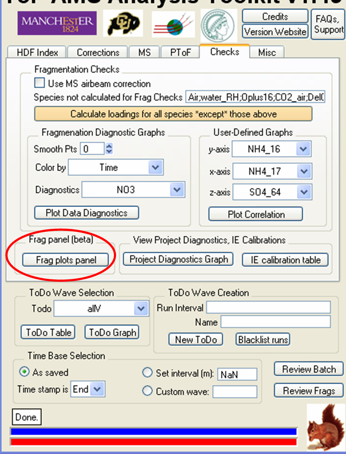
Button for the frag panel in 1.50+
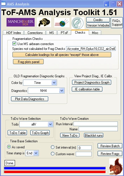
Button for the frag panel in 1.51+
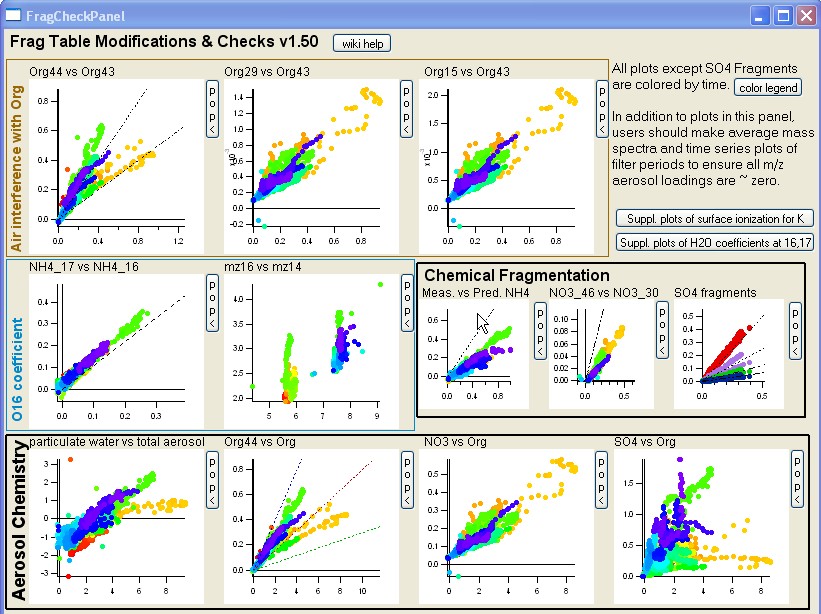
New frag panel


Above are pictures of the button in the AMS panel and the resulting frag check panel on some ambient data. Text below will discuss selected default frag entries and modification results on a sample data set.
Air Fragmentation Patterns
Most of the necessary adjustments to the default frag table have to do with air interferences. The top left 3 graphs in the frag check panel deal with air interferences.
Frag_CO2[44]
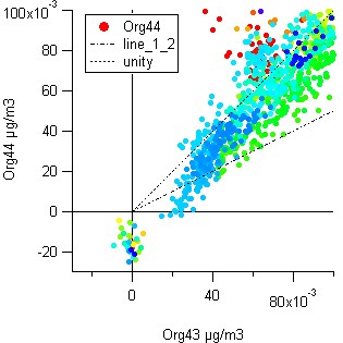
Before default frag change
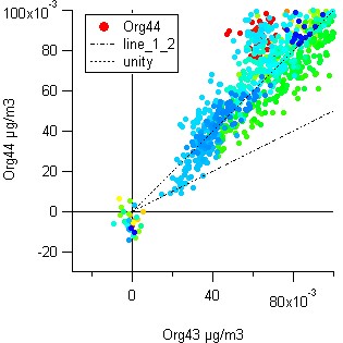
After default frag change


Task for user: Change default at frag_CO2[44] = 0.00037*1.36*1.28*1.14*frag_air[28]
Data should go through origin (or should trend to go through the origin); users should change the 0.00037 coefficient.
Impacted frag entries: frag_air[44]=frag_CO2[44] and frag_organic[44]=44,-frag_air[44]
The frag_CO2[44] coefficient is a combination of a number of factors including:
- 1. the mixing ratio of CO2 in air (0.00037 = 370 ppm of CO2);
- 2. the RIE of CO2 from the literature (1.36);
- 3. the reciprocal of the fraction nitrogen in air (1.28), and;
- 4. a correction for mz15 fragmentation of nitrogen (1.14).
The graphs show the Org44 vs Org43 correlation plot with a 1:1 and a 1:2 lines for reference. Org 43 is a purely organic signal. The amount of 44 (mostly CO2) signal which is due to gas phase CO2 and the amount of aerosol phase CO2 (and other small aerosol contributions at 44) needs to be adjusted to reflect sampling conditions. Users should change the 0.00037 coefficient to make the data points intersect the origin, regardless of organic aerosol type or origination. If users have an external measurement of gas phase CO2, a time dependent frag entry can and should be used (see wiki explanation and syntax). On some unusual occasions it is appropriate that the RIE term also be modified, but typically changes to the single 0.00037 term is sufficient.
In the example above, a higher value of Org44 is needed for the trend in the data to go through the origin. Thus a smaller value of the gas phase CO2 coefficient is needed. In the example above a change was made from the 0.00037 default to 0.0033.
Frag_air[29]
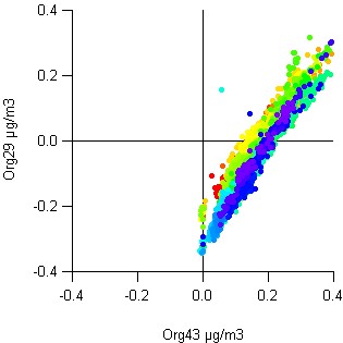
Before default frag change
After default frag change


Task for user: Change default at frag_air[29]= 0.00736*frag_air[28]
Data should go through origin (or should trend to go through the origin); users should add a correction factor near 1.
Impacted frag entries: Frag_organic[29]=29,-frag_air[29]
The graphs show the Org29 vs Org43 correlation plot. Org 43 is a purely organic signal. Depending on the threshhold setting and possible saturation effects, the amount of N15N at m/z 29 detected by the system may be slightly different than that predicted purely by an isotopic factor.
In the example above a higher value of Org29 is needed; thus a smaller value of the gas phase m/z 29 is needed. Inn the example above a the modified frag entry was 0.91*0.00736*frag_air[28].
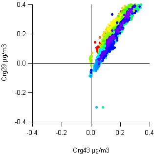
Frag_air[15]
Before default frag change
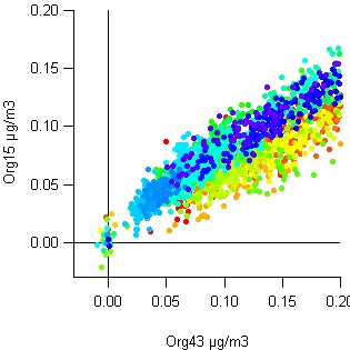
After default frag change


Task for user: Change default at frag_air[15]= 0.00368*frag_air[14]
Data should go through origin (or should trend to go through the origin); users should add a correction factor near 1.
Impacted frag entries: frag_organic[15]=15,-frag_NH4[15],-frag_air[15]
The graphs show the Org15 vs Org43 correlation plot. Org 43 is a purely organic signal. Depending on the threshhold setting and possible saturation effects, the amount of 15N at m/z 15 detected by the system may be slightly different than that predicted purely by an isotopic factor.
In the example above a slightly smaller value of Org29 is needed; thus a higher value of the gas phase m/z 15 is needed. In the example above the frag_air[15] entry was changed to 1.2*0.00368*frag_air[14].
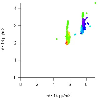
Frag_O16[16]
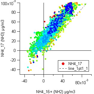
Before default frag change
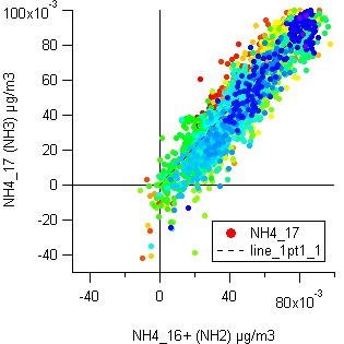
After default frag change
step change


Task for user: Change default at frag_O16[16]=0.353*frag_air[14]
Data should go through the origin (or should trend to go through the origin) for the NH4_17 vs NH4_16 plot and data should go through the trend of the mz16 vs mz14 plot with an intercept of zero.
Impacted frag entries: frag_air[16]=frag_O16[16],frag_RH[16] and thus frag_air[17] and frag_air[18] and thus all frag_water entries; frag_NH4[16]=and thus frag_NH4[15] and frag_NH4[17]
Two graphs above show the frag_NH4[17] (NH3+) vs frag_NH4[16] (NH2+) correlation plot with a 1:1.1 line for reference. The two ammonium chemical fragments should be correlated. Frag_O16 indicates the amount of gas phase signal due to O+ or a doubly charged O2 ion. Two approaches can be used to determine this amount. One approach is to find the correlation of NH3 to NH2 (NH4_17 and NH4_16); the intercept should trend to the origin. Alternatively one can assume a constant ratio between mz16 and mz14 (predominantly O+ and N+) and determine the slope of this line with an intercept of zero.
In the example above the mz16 vs mz14 plot doesn’t show a well defined slope; the grouping of the data into two clumps, separated in time, indicates a systematic change in the behavior of the difference signal of at m/z 16 and 14. In this example, this plot is not useful for determining the frag_O16 correction.
The NH4_17 vs NH4_16 plot shows that NH4_16 may be slightly too small. To make it larger, we must subtract a smaller value for frag_air[16]. In the example above the frag_O16[16] entry was changed to 0.96*0.353*frag_air[14].
Other Fragmentation Table Adjustments
Adjust Frag_Org[39]
The Squirrel default frag_organic wave doesn't attribute any organic signal at m/z 39. This is because there is an interference from K+ at that m/z, which can be very large and variable in some datasets. However in many datasets, after checking the HR data in PIKA and verifying that K+ is negligible for your dataset, one can set Frag_Org[39] = 39.
Water Fragmentation Pattern
Water typically dominates the closed spectrum so the signals at m/z's 16, 17, and 18 can be used to determine the fragmentation pattern for water.
Previous versions of this frag table modification wiki included discussion on modifying the water coefficients. However since particle water is generally not quantifiable in the AMS, it is no longer recommended to perform these corrections. If a user does opt to modify the fragmentation coefficients for water (at m/z 16 for O+ and m/z 17 for OH) the water fragmention pattern is used in four places in the frag table and the coefficients MUST be changed at each fragment when altering the default coefficient values .
Modifying Nitrate Fragment (frag_org[30])
The default apportionment of m/z 30 is:
frag_nitrate[30]=30,-frag_air[30],-frag_organic[30]
frag_organic[30]=0.022*frag_organic[29]
frag_air[30]=0.0000136*frag_air[28]
The current value for Frag_Org[30] is based on isotopes of Frag_Org[29] (mostly CHO+). Some non-nitrogen-containing organic material could also be present at 30 (CH2O+), making the isotope attribution too low for Frag_Org[30]. In some cases, the ratio between NO3_30 and NO3_46 can be forced to be the same as for ammonium nitrate (from the calibration). This would be reasonable if there are no other types of nitrate present, such as sodium, calcium, or organic nitrate which tend to have a higher 30/46. Where possible, high resolution analysis can sort this issue out. In the absence of high resolution data, the attribution of 30 should be something for the data analysis person to decide.
Modifying Sulfate Fragments
Squirrel experiments contain three fragmentation waves that have to do with aerosol sullphate: frag_SO3, frag_H2SO4, and a 'composite' frag_sulphate which contains entries from bothe frag_SO3 and frag_H2SO4. For almost all users the distinction between frag_SO3 and frag_H2SO4 entries is not important, frag_sulfate is the frag wave that is used for the sulfate (SO4) species. The fragmentation pattern for sulfate, between SO+, SO2+ etc, is not relevant for most analyses.
The correlation plot between the sulfate fragments (mz64:mz48, mz80:mz48, mz81:mz48, and mz98:mz48) should have linear relationships. Although the linearity of data is important, the exact slopes of lines are unique to each instrument (these slopes can also be compared with (NH4)2SO4 calibration if required). To check for the presence of organic sulfates, the correlation of any deviation from linearity with organics can be investigated.
Modification of the sulfate fragments can be made, but are not often necessary (the possible exception being when sulfate is low and organics are high). Any adjustments can be made at frag_org[80] and [81]. If there is evidence of MSA, organo-sulfites or organo-sulfates in the aerosol, the sulfate fragments will need to be adjusted.
Evaluate Ammonium Balance
While not a frag table issue, an examination of the ammonium balance often happens shortly after frag table modifications have been performed. The measured vs predicted NH4 correlation plot can assist with this determination. The formula for the predicted amount of NH4 is:
NH4_predict = 2*(18/98)*SO4 + (18/63)*NO3 + (18/35)*Chl
where the fractional amounts correspond to the molecular weights of the relevant species and the SO4, etc values are the time series values.
Make average mass spectra plots of filter periods to double check fragmentation table modifications
It is advised that users collect filter measurements frequently during their ambient sampling. Creating todo waves of only the filter period runs and generating average mass spectra is a very good way to ensure that the frag table adjustments have been properly made. All mass spectra sticks from each of the 5 main aerosol species should have magnitudes of approximately zero.
Generate time series and average spectra of unit-resolution data
Choose preliminary CE from observed composition and accumulated AMS experience
The data processing steps described above produce a concentration of each species (as measured by the AMS) from first principles. E.g. 5.2 ug m-3 of sulfate at 4:00-4:05 PM. In the first studies using the AMS for ambient data (Jimenez et al., 2003; Drewnick et al., 2004; Alfarra et al., 2004) it was observed that the AMS concentration had the same structure in time as for other collocated instruments (PILS species, TEOM mass, SMPS volume), but that it was low. Comparing individual species such as sulfate it was found at the AMS concentrations needed to be multiplied by ~2 to match the concentrations measured by other quantitative instruments. This is normally expressed as a collection efficiency CE = 0.5.
Early on it was thought that CE < 1 arose from excessive broadening of the particle beam at the exit of the aerodynamic lens inside the AMS, leading to some particles not hitting the vaporizer and thus not being detected. This led to the development of an automated Beam Width Probe (BWP, Huffman et al. 2005). However the use of the BWP in many ambient studies (summarized in Salcedo et al., 2007) has shown that this is not a problem.
Tim Onasch et al. during the Ron Brown 2004 study showed convincingly (by comparing PToF and light scattering particle pulses) that the cause of CE < 1 was particle bounce at the vaporizer. Huffman et al. (AS&T 2005) expressed CE = E_b * E_L * E_s to clearly separate the different effects that may reduce the signal reaching the AMS vaporizer. Only E_b is due to particle bounce.
The current status (as of June 2007) of the E_b issue is as follows:
(a) Aerodyne has tried several new vaporizer designs in an attempt to reduce or eliminate bounce. However these have not been successful so far.
(b) For that reason, at present CE is estimated based on the observed composition and phase of the particles, and verified based on intercomparisons with other quantitative instruments.
Fortunately CE ~ 0.5 has been found to hold in most field studies, including those dominated by sulfate and/or oxygenated organics (OOA). Laboratory studies can be more variable depending on the particle phase and volatility used. Known deviations from CE ~ 0.5 include:
(a) Liquid organic particles or particles with a large liquid coating, which are collected with CE = 1. Note that OOA and solid organic particles do bounce (e.g. SOA measurements by Bahreini et al., 2005).
(b) Sulfate-dominated particles can be collected with CE > 0.5 when the particles are acidic, i.e. there is not enough NH4+ to neutralize all the sulfate. This has been seen in many field studies. Based on the Onasch et al. measurements in 2004, CE = 0.5 until the sulfate is in the form of bisulfate, at which point CE increases linearly and reaches CE = 1 for H2SO4.
(c) Particles dominated by ammonium nitrate (NH4NO3 > 50% of the mass). In this case CE also increases, which can be parameterized in the same way as (b), but with the X-axis being the NH4NO3 mass fraction.
(d) Particles with high water content that retain significant water in the AMS lens. This was pointed out by James Allan in his 2004 JGR paper, and also shown by Matthews et al. with laboratory particles (AST, 2008). However organic-dominated ambient particles do not seem to pick up enough water to drive their CE to 1 using this effect (e.g. per experiments from Tim Onasch and Tim Bates in the Ron Brown during ICARTT 2004). For this reason this method has not been pursued, and the use of a dryer in front of the AMS is highly recommended to remove this potential composition-dependent effect on E_b.
(e) (a)-(d) above assume internally mixed particles, which is very often the case for ambient data. However if you see a particle size distribution mode that is clearly externally mixed, it will have its own CE. We have seen this sometimes with NH4NO3 condensation into small particles in the early morning in the Eastern US, when those particles can have E_b ~1 even though the accumulation mode has E_b ~ 0.5. It can also happen when a fresh power plant or volcanic plume with lots of acidic sulfate is embedded in a more aged aerosol, and this has been seen in multiple aircraft experiments.
IMPORTANT NOTE: disagreements between concentrations from the AMS and other instruments can arise for many other reasons than variations in Eb. For example the AMS user may have made mistakes in its inlet setup or lens alignment (causing large particle losses), or the threshold setting, the IE calibrations or IE/AB corrections, or in determining the single ion, or in other AMS data processing procedures. And even more often in our experience, other instruments have problems (of functioning, software, or inlets) that may not be noticed, especially standard instruments that don't receive much attention during a campaign (such as an SMPS or OPC). We have seen every type of quantitative instrument produce wrong concentrations at least once in the field (including PILS, TEOM, etc.). If you think you are seeing a CE that is changing all over the place, almost certainly the problem is somewhere else in the AMS or other instruments. The CE / E_b SHOULD NOT BE THE WASTEBASKET OF ALL DISAGREEMENTS. Rather CE should be chosen based on the composition-based rules above, and remaining disagreements should be investigated by looking at all aspects of the AMS and of other instruments.
Look a MS and size distributions of very large outliers, blacklist if appropriate
Work up comparisons of total mass and volume with other instruments
Make size distributions for a handful of periods with good signal
Work up comparisons of size distributions for those same periods with other instruments
Reevaluate CE choice based on intercomparisons
Start looking at the scientific questions of interest
Mission Diagnostics Plot
The mission diagnostics plot (MDP)is useful to diagnose both instrument performance during a field campaign and also to more easily determine where various corrections to the data are required. Throughout the above discussions, the user is prompted to add data to this plot at various steps within the analysis process. It is STRONGLY suggested that a MDP be produced for every data set. In Squirrel versions 1.39 (?) and above, this plot is created using various user interfaces within the data analysis software. However, for analysis conducted in earlier versions of the software, this plot must be produced manually.
Sample image of mission diagnostic plot (produced from SOAR1 data). In this plot, calibration data are represented by circles and Squirrel data are represented by lines.

Determining Precision Directly from Field Data
See the following procedure adopted by NASA as part of the Tropospheric Airborne Measurement Evaluation Panel (TabMEP) process.
Reporting your data
At a gathering of many European AMS users in May, 2009, it was suggested that users routinely report their data with supplemental information about the measurement configuration and analysis. The list of suggested supplemental fields is:
- AMS_Type: C, V, or W, and ionization type if not EI
- AMS_SamplingTime: length of time of typical run, and any other info (2 minute data saving alternating V and W mode)
- AMS_LensType: standard, high throughput, etc
- AMS_LensPressure: typical lens pressure
- AMS_FlowRate: typical flow rate
- AMS_PrsTempFlowCal: P & T of room the AMS was in during the flowrate calibration, i.e. 1 atm, 30 C, 20 cc/min
- AMS_STPConversionFactor: conversion factor for STP (273K 1 atm)
- AMS_IEOverAB: description of IE/AB ratio used for data processing (can be a single value or several) If using a single value, report the IE/AB ratio as calculated from the IE and AB values used in the airbeam correction.
- AMS_RIENH4: description of the RIE used in data processing for the Ammonium calibration
- AMS_CE: description of the CE value used (e.g. single value or based on acidity etc.)
- AMS_PMCut: PM cut on inlet e.g. Size cut for inlet line at 2.5 micrometers
- AMS_InletRH: inlet dried or ambient (how?) Inlet RH < 40% using nafion drier
- AMS_LocalToUTCTime: for ground-based station, time relative to UTC e.g UTC + 2h
- AMS_RelatedInstrumenationInfo: i.e. other instruments that shared the inlet
Reporting in ICARTT Format
Information and Software for the ICARTT file format can be found here