1. Start with topography (see below). This was reprojected from a 30' dataset; the pixels are about 2.5 km apart. You can get the original HDF file.

   

2. To make shaded relief from this, the following can be entered in the notebook:

   shade=LTmask(kernel(topo,slmask)/dx - sin (dtor(el)),0)/(1. - 1./(kernel(topo, slmask)/dx - dsin(dtor(el))))

   Where el is the elevation of the sun over the horizon and dx is the spacing between pixels in the same units as topo (arbitrary if you are not doing topography) and slmask is a 3x3 kernal (a 3x3 matrix)

   [ 0 0 0 ] slmask = [ 0 -s1+s2 s1 ] [ 0 -s2 0 ] where s1 = sin(az)*cos(el), s2=cos(az)*cos(el) and az is the azimuth of the sun (relative to the top ("north")--this is using a 3 point estimate for slope; you could revise this in several ways to get 5 point or 9 point estimates of the slope (I use 3 point, even though it sort of offsets things, because it will preserve as much slope info as possible). The use of the LTmask is to prevent shadows from having negative values.

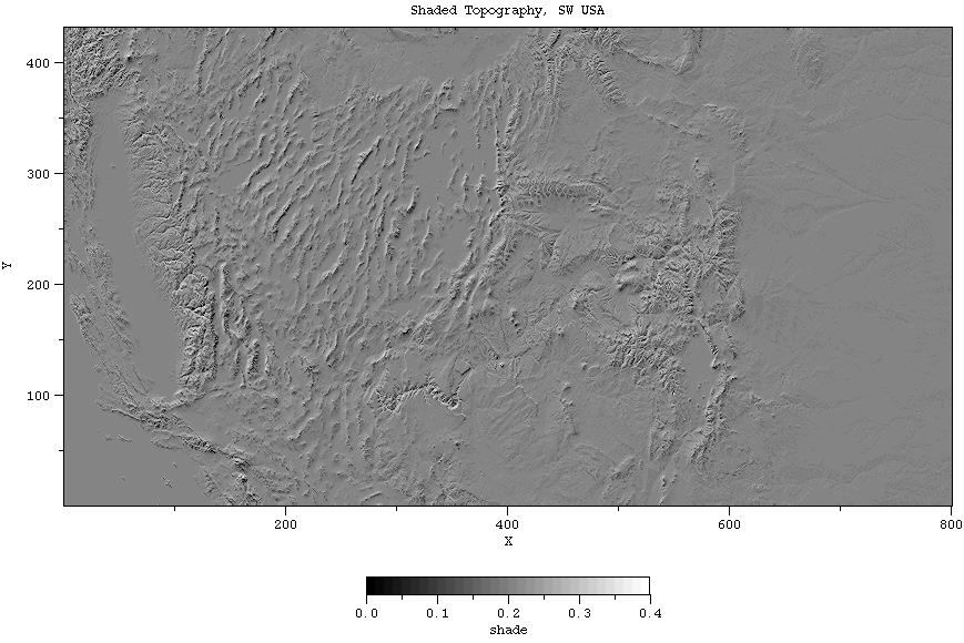
   For an example here, shade from 330 at an elevation of 15 degrees to get

   s1 = sin(dtor(330))*cos(dtor(15)) = -0.482963

   s2 = cos(dtor(330))*cos(dtor(15)) = 0.836516

   shade=LTmask(kernel(topo,slmask)/2500 - sin (dtor(15)),0)/(1. - 1./(kernel(topo, slmask)/2500 - sin(dtor(15))))

   This will produce the image below; you can get the original HDF file of the mask or the file of the shaded relief and play with it.

   

3. You then can combine this with the topography to get a shaded topographic map or with something else to "drape" that over the topography. For instance, you could drape the geoid (the difference between sea level and a reference ellipsoid) over topography. The geoid HDF file is also available. To combine shade and some other file representing the same area, say data, assign the top x bits to "topo" and the remaining bits to "shade"; usually I use 4 or 5, though if you only want 8 colors and detailed shading, 3 might work well. You could do this in two parts and make some complicated assignment of both shading and topo to their bits before combining, but the simplest way (linear combination of both) runs something like this:

   shdata = 2^(8-x)* int(2^x*(data-min(data))/(max[data] -min[data]+delta)) + int(2^(8-x) * (shade - min(shade))/(max(shade) - min(shade) + delta))

   where delta is to prevent things from slopping over; a mask will work, too. so if we use x=5, then

   shdata=8*int(32*(data-min(data))/(max[data] -min[data]+delta)) + int(8 * (shade - min(shade))/(max(shade) - min(shade) + delta))

   masks could be used to trim out unwanted things and prevent bleeding into other parts of the image. Since 0 and 255 are not permitted values, you have to be careful of this. For our example, we will split shading and data equally, giving each 4 bits:

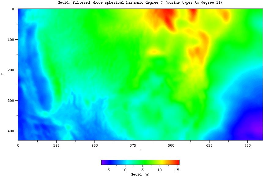
   shaded_geoid = 16*int(16*(Geoid-min(Geoid))/(max(Geoid) -min(Geoid)+0.01)) + int(16 * (shade - min(shade))/(max(shade) - min(shade) + 0.001))

   Here's the raw file before the shading was applied:

   

   Now if you merely make an image of the shaded file (available as an HDF file) with a standard color palette, you won't see anything special, except that your image now has become a bit banded. You need a special color map; you can use my little code ShadePalette (part of the Shading with Transform code collection) or edit your own in the Color Editor in the View Utility. The idea is to vary the hue and saturation with the upper bits and the lightness with the lower bits, as this snapshot of the Color Editor illustrates:

   

   This is for a file using the 8 bits equally for color and shading and modifying the Rainbow palette shipped with Transform. A collection of some of the color palettes built upon 2 of the color palettes shipped with Transform can be had as HDF files. For our example, this looks like this when we use this palette:

   

   You'll note that the shading degrades the smoothness of the colors assigned to the geoid, owing to the smaller number of colors available for the geoid intensity. This can work to your advantage as these are, in essence, contours and can be assigned to useful values, if desired, when assigning the geoid (or other data) to the high order bits.

4. Of course, a fairly popular thing to drape over shaded relief is topography itself, forming a shaded topographic map. Using my own palette modified from the Earth-Land palette used for the topography plotted at the top of this page, I get this image:

   

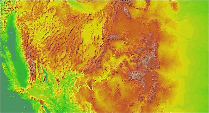
   In particular, if you compare the larger JPEG file with the original topo plot, you can see a lot of the details of the topography that otherwise are hard to pick out. This plots uses 5 bits for topography and 3 for shaded relief.

1761 visits from Tue, Apr 21 1998 17:07 to Apr/ 6/02 19:34