California
Creepmeters
Roger Bilham, Naia Suszek and Sean Pinkney
CIRES & Department of Geological Sciences
University of Colorado Boulder CO 80309-0399
INTRODUCTION
A handful of faults in California manifest some form of surface creep: afterslip, episodic slip, steady slip, or triggered slip. Creep can be considered a proxy for shear strain applied to a fault, although its rate is sensitive also to fault normal stresses, and variations in the frictional properties of the near-surface fault. Creepmeters afford a view of fault activity with micron precision, at rates of up to 5 mm/minute, though creep rates on most California faults are typically less than a few mm/year. This article summarizes the current status of creepmeters in California and their contribution to the study of plate boundary slip. We describe two new creepmeters: one designed for autonomous year-long deployment with 10µm precision, and another with mm precision and 3 m range designed to capture pre-seismic, co-seismic and afterslip associated with seismic rupture. We discuss a third system that provides both high resolution and large range. The anticipated availability of displacement and strain-fields applied to California faults following the successful implementation of the Plate Boundary Observatory (PBO) promises new insights in the mechanism of creep, and its potential utility in the study of the earthquake cycle.
Fig. 1. The depth to which creep extends, and
the applied strain rate, determines the creep rate of a fault. A creepmeter
monitors fault slip between two monuments on either side of a fault as the
varying displacement of the free end of an inextensible rod.
Creep occurs in the shallow parts of certain faults (Figure 1). Its rate is proportional both to the depth to which it occurs, and to the rate at which shear stress is applied to the fault (e.g. Savage and Lisowski, 1992). The depth to which creep occurs is determined by the physical properties of the fault zone, but it is partly proportional to the fault-normal stress applied to the fault, and to the fault-normal stress. Thus a change in creep rate may accompany either a change in fault-parallel shear stress or a change in fault-normal stress applied to a creeping fault. Creeping faults are a proxy for applied strain. For example, strain released by the Loma Prieta earthquake modified the creep rate on the Hayward, Calaveras and San Andreas faults in succeeding years (Lienkaemper et al., 2001). Similarly the strain changes that accompanied the Landers earthquake sequence modified creep rates in southern California (Lyons and Sandwell, 2002).
Creep reduces the strain energy near a fault zone
potentially available to drive a future earthquake. The relation between shear stressing rate ![]() , and surface creep rate
, and surface creep rate ![]() for a long fault
locked between an upper depth d
and lower depth D is
for a long fault
locked between an upper depth d
and lower depth D is
![]()
(Savage and
Lisowski, 1993). For the Hayward fault ![]() ≈ 0.2 microradians per year where µ is the rigidity of the
crust (≈30 Gpa). The rate of slip of the fault below
depth D=10 km is assumed to equal the geologic slip rate on the fault. Hence if
the depth of creep (the upper locking depth), remains constant, the creep rate is related to the
stressing rate. A creep rate of 5
mm/yr corresponds to a locking depth of 5.3 km.
≈ 0.2 microradians per year where µ is the rigidity of the
crust (≈30 Gpa). The rate of slip of the fault below
depth D=10 km is assumed to equal the geologic slip rate on the fault. Hence if
the depth of creep (the upper locking depth), remains constant, the creep rate is related to the
stressing rate. A creep rate of 5
mm/yr corresponds to a locking depth of 5.3 km.
If the locking depth remains constant, changes in the rate of creep on the fault indicate changes in strain rate applied to the fault. However, a change in the locking depth may also accompany changes in fault zone rheology, or fault-normal stress. The interpretation of creep as a proxy for applied strain has most utility in locations like the northern Hayward fault, where stick-slip behavior appears to be absent. A creepmeter across such a fault acts as strain-meter that samples strain averaged over many km along the fault and several km from the surface to the locking depth. In this sense a creepmeter is less sensitive to local sources of strain "noise" than is a borehole strainmeter. In practice other forms of noise exist in the fault zone that may be difficult to characterize (e.g. surface soil moisture changes).
Four types of aseismic slip process have been quantified on surface faults. A fifth form of creep – precursory slip - remains enigmatic. In each process surface slip occurs without the radiation of seismic energy:
 Steady-state creep: Parts
of the San Andreas fault in central California and the Hayward fault are
observed to slip linearly with time.
The slip rate in some locations (e.g. the northern Hayward fault) is
linear to within 1% over many years.
Steady-state creep: Parts
of the San Andreas fault in central California and the Hayward fault are
observed to slip linearly with time.
The slip rate in some locations (e.g. the northern Hayward fault) is
linear to within 1% over many years.
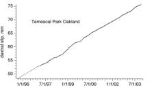
Fig. 2. Creep at Temescal Park on the Hayward fault near Oakland exhibits approximately linear creep at 3.5 mm/year. The creep signal here sampled by a 148-m-wide alignment array is 3.9 mm/year (Galehouse and Lienkaemper, 2001), similar to the rate sampled by the 15-m-wide aperture of the creepmeter.
Creep events: Creep events occur when slip accelerates over a few hours or days. These events start impulsively with slip rates of up to a few mm per minute and asymptotically approach a low creep rate within a few hours or days (Bilham, 1987). On some faults creep events are superimposed on a steady background creep-rate suggesting that steady slip may occur in the uppermost surface layers, with creep-events occurring as stick-slip events at deeper depth (Bilham and Behr, 1992). Creep events have been observed to accompany, or follow slow earthquakes at depth (Linde et al., 1992).
Fig. 3 An 8 mm amplitude double creep event on
the Superstition Hills fault near Imler Road (16 July 1991) with a duration of
2 hours. Sample interval is 1 minute (from Bilham and Behr, 1992)
Afterslip: When fault creep occurs as afterslip, it
causes surface slip to rise asymptotically to match coseismic slip at
depth. It is probable that no
surface slip occurred during the mainshock of the 1987 Superstition Hills
earthquake, and all surface slip (>1 m) developed subsequently (Bilham,
1989), 90% of it occurring in the three years following the earthquake. The logarithmic decay of slip observed
in Parkfield in 1966 suggests that surface slip on the San Andreas fault was
also small during the mainshock (Smith and Wyss, 1968), but approached coseismic
slip amplitudes in the following few years.
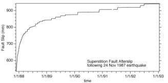
Fig. 4. Three years of afterslip on the
Superstition Hills fault.
Afterslip is observed to be formed from a sequence of creep events
imposed on a steady background slip.
The two processes appear to be caused by creep occurring at different
depths. Episodic creep occurs in a transition zone below a shallow part of the
fault zone that slips steadily between creep events (Bilham & Behr 1994).
Triggered slip: Earthquakes on nearby faults have been found to increment surface slip on creeping faults (Allen et al., 1972). Triggered slip is initiated at the time of passage of large amplitude surface waves (Bodin et al., 1994). Both dynamic and static stresses appear responsible for triggering surface faults (Kilb et al. 2000; Gomberg et al., 2001; Du et al., 2004).
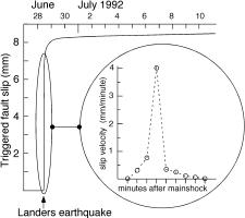 Fig. 5. Slip triggered on the Superstition
Hills Fault at Imler Road by the Landers earthquake. Triggered slip occurred
during the passage of Raleigh waves from the Landers mainshock (from Bodin et
al, 1994).
Fig. 5. Slip triggered on the Superstition
Hills Fault at Imler Road by the Landers earthquake. Triggered slip occurred
during the passage of Raleigh waves from the Landers mainshock (from Bodin et
al, 1994).
Precursory creep: A fifth form of creep – precursory slip – has yet to be quantified on a surface fault. It may have preceded the 1966 Parkfield earthquake, as suggested by the anecdotal breakage of a water pipe across the surface fault some eleven hours prior to the earthquake. The possibility that slip accelerated prior to the earthquake is considered an important motivation for monitoring fault creep. However, the logarithmic afterslip decay curve at Parkfield Smith and Wyss, 1968) indicates that slip was small at the time of the 1966 aftershock suggesting that if any precursory accelerated creep occurred, its amplitude was probably small.
Creepmeters
Steady creep on the San Andreas fault system has been documented for more than four decades (Tocher, 1960; Steinbrugge and Zacher, 1960). Creep was discovered as surface afterslip in Parkfield in 1966, and as triggered-slip in the Coachella Valley in 1968. In 1970 creep was reported to have occurred on the Anatolian fault near Ismet Pasa (Ambraseys, 1970), and triggered slip has been noted subsequently (Dogan et al., 2003). Surface creep also occurred on the Xianshuihe fault in the form of afterslip following the 1973 Luhuo earthquake (Allen, 1991; Bilham, 1992), and on the Chihshang reverse fault in eastern Taiwan (Lee et al., 2001). Minor afterslip was reported following the Dasht e Bayaz earthquake of 1968 ( King et al., 1975) and across the Nahan thrust in the Himalaya (Sinvhal et al., 1973).
Soon after the discovery of fault creep in 1956 in
California, a program of
measurements using theodolites and dial gauges instruments was initiated to
quantify the slow aseismic movement of surface faults (Yamashita and Burford,
1973; Nason et al., 1974; Schultz, 1989).
The dial gauge devices used invar rods, installed obliquely at 45° and
at shallow depth across the fault.
Early creepmeter sensors used a filament wound around the shaft of a
low-friction potentiometer to provide an electrical measure of creep suitable
for telemetry or local recording, but these simple sensors were subsequently
replaced with zero-friction LVDT's (Linear variable differential transformers).
Twenty-one of these early creep-meters continue to be operated by the USGS
using telemetry to bring the data to Menlo Park. Several creepmeters have
operated briefly in post-seismic investigations (Bilham, 1989; Bodin et al,
1994; Behr et al, 1994, but with the exception of five new creepmeters on the
Hayward fault (Bilham and Whitehead, 1997) no new permanent creepmeters have
been installed,
 Fig. 6
Schematic views of four creepmeter piers in use in California. Three helical piers (one driven
vertically and two at 45° away from the fault) are used for each pier in the
Hayward creepmeter array. They meet at a point and are welded roughly 1 m below
the surface. An experimental
inclinometer system was installed in Fremont on the Hayward fault whose tilt at
every 50 cm segment of the borehole may be monitored using a force–feedback
tiltmeter (Bilham1995). Most creepmeter piers, however, consist of augered
pillars cemented in place.
Hand-driven reinforcing bar is typically used in afterslip studies. The vertical piers of a 30°
-oblique and 30-m-long creepmeter are less than 7.5 m from the center of a
1-m-wide fault. Since most
creeping faults are several meters wide the mounts can easily be within the
shear-strain-field of the creeping fault unless special care is taken to
lengthen the creepmeter sampling interval.
Fig. 6
Schematic views of four creepmeter piers in use in California. Three helical piers (one driven
vertically and two at 45° away from the fault) are used for each pier in the
Hayward creepmeter array. They meet at a point and are welded roughly 1 m below
the surface. An experimental
inclinometer system was installed in Fremont on the Hayward fault whose tilt at
every 50 cm segment of the borehole may be monitored using a force–feedback
tiltmeter (Bilham1995). Most creepmeter piers, however, consist of augered
pillars cemented in place.
Hand-driven reinforcing bar is typically used in afterslip studies. The vertical piers of a 30°
-oblique and 30-m-long creepmeter are less than 7.5 m from the center of a
1-m-wide fault. Since most
creeping faults are several meters wide the mounts can easily be within the
shear-strain-field of the creeping fault unless special care is taken to
lengthen the creepmeter sampling interval.
The most important improvement in
creepmeter design in the past decade has been the introduction of deep
anchors. These are costly (≈$6k)
but only with their introduction has it been possible to obtain reasonable
immunity to soil expansion and contraction effects (<1 mm/year) caused by
variations in soil moisture.
Two types of end monument have been tested: deep vertical pillars whose
lateral offset can be monitored
relative to their base, and helical piles driven in the form of a buried
tripod. Both mounts terminate
beneath the surface and define the attachment points of the creepmeter on
either side of the fault. The assumption in both is that at some depth,
horizontal displacements caused by random and systematic soil motions are
negligible. An advantage of the drilled pillar approach is that it effectively
monitors the decay in these lateral motions with depth (Bilham, 1993; 1997),
however, its slender pillars (30 cm diameter and 30 m deep) may be deflected by
lateral forces in the near surface.
These motions may occur between inclinometer measurements, although they
could, in principle, be measured
using a continuous recording tiltmeter.
Helical piles have the benefit that if the screw-helices that terminate the base of the piles are sufficiently deep (e.g.≥10 m), lateral motions of the attachment points of the creepmeter are negligible. Helical piles tend to remain stable even under large loads. They were developed as supports for rail- and road- bridges crossing rivers, or as pilings for ocean-front piers. Helical piles are driven into the ground by powerful hydraulic rotary torque motors. Five-cm-square, 3-m-long bars are added incrementally until the helix refuses to drive deeper. In some helical piles a 3 inch galvanized steel pipe is used instead of 2 inch square-section bar.
An assessment of noise in the Hayward creepmeters suggests that engineered piers contribute less than 1 mm/year of noise to the creep signal in the Bay Area ( Bilham 1987) demonstrating that even in expansive clay environments reasonable immunity to moisture signals can be obtained. Random noise levels in the creepmeter data are of the order of 0.2 mm/yr but it is difficult to evaluate the contributions from flooding and thermal effects on the creepmeter rods. Despite the advantages of engineered mounts, the five Hayward fault creepmeters alone are equipped with helical piers. Unfortunately most of the aging California creepmeter array operates with shallow anchors with poor immunity to surface moisture changes.
Length-standards
and rods
New materials are now available for the length-standards that cross the fault. While invar rods remain in use, they are heavy and can corrode. The availability of quartz fiber, glass fiber and carbon fiber rods provides similar low thermal coefficient materials with densities almost five times lower, and a superior resistance to corrosion (Table 1). These tough, low-density, length-standards can slide through buried pipes with reduced stick-slip behavior. While suspended catenary wires boast zero friction when installed within large diameter buried tube, they are impractical for wide fault zones requiring installations whose lengths exceed 20 m. This is because the resonant frequency becomes unmanageably low as the wire length increases. Longitudinally stiff rods in telescopic plastic jackets can be used in fault zones more than 100 m wide although the longest creepmeter currently in use is 33 m long. Stick-slip behavior of up to 0.5 mm is manifest in rod type creepmeters, aggravated by the entry of grit into the guide tubes. Such behavior can be reduced using rolling supports or flexure guides.
Table 1 Properties of
six-mm-diameter rods used in
creepmeters
Material Thermal Coefficient of linear expansion cost/m
Invar 0.93-1.0 x 10⁻⁶/°C $10/m
Glass fiber composite 6.5 x 10⁻⁶/°C $7/m
Quartz fiber (Teflon-coated) 8.7 x10 -6/°C $15/m
Quartz fiber composite -0.64 x10 -6/°C $15/m
Carbon Fiber composite 0.32- 0.65 x 10⁻⁶/°C $17/m
Transducers
Sensors used in present creepmeters are invariably LVDT's since these can operate submersed underwater for extended periods; a typical condition when the water table rises during the rainy season in California. Capacitative sensing digital calipers were used in afterslip studies in southern California but these proved unsuitable in wetter climates. Recent developments in low power LVDT's permit the autonomous operation of creepmeters for prolonged periods.
Micro-power
creepmeter
A creepmeter capable of operating from alkaline cells for a year is an appealing instrument where vandalism is endemic (most of the world, unfortunately), or where no surface expression of a buried instrument is permitted (e.g. National Parks). A micro-power creepmeter can be buried completely and its data retrieved annually, or when needed.
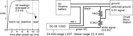
Fig. 7. Circuit diagram for a low power
creepmeter. The measured
transducer rise-time in switched operation is approximately 5 ms (left),
resulting in an average power
consumption of 11 µW at 1 sample per minute. The LVDT is calibrated ±0.9 volt beyond its 25.4 mm linear
range to utilize the full 34 mm range of the transducer. The batteries and
recorder are sealed within a 10 cm diameter PVC tube, and the LVDT body is
coated with silicon grease to permit prolonged underwater operation.
The micropower creepmeter is based on a DC-SE 1000 Schaevitz 25.4-mm-range transducer that operates from a single sided 9 V power supply at 6 mA. To prolong battery power the LVDT is switched on 10 ms prior to data acquisition and is powered off for most of the time (Figure 7). Switching is controlled by an Onset Microstation 12-bit data logger. The data logger reads 32 samples in the succeeding 2.5 ms and stores the average. Temperature (0.02°C resolution) and displacement (6µm resolution) can be measured once per minute for 170 days, once every two minutes for 340 days, or longer at lower sampling rates. The Onset data logger includes a 512 Mb non-volatile memory. Although AA batteries can power the LVDT for a year, six D-cells are typically deployed.
The range of the transducer is extended by 25% (i.e. by ±4.5
mm) beyond its linear 25 mm range by calibrating the LVDT in the laboratory
prior to deployment. The batteries
and data logger are installed in a 10 cm diameter PVC tube with a rubber lid
that is sealed and buried with the LVDT sensor. Since the carbon fiber or invar rod is buried at 30° to the
fault and fastened rigidly to the ground on the far side of the fault,
displacements measured by the transducer
must be increased by 15% (1/cos(30°)) to convert them to displacements
parallel to the strike of the fault.
Hence the operating range of the transducer is effectively 39 mm, and
the corresponding strike-slip, least-count resolution is 10 µm. This displacement corresponds to a
temperature increase of 1°C in a 10 m long carbon fiber rod. Annual thermal variations at 30 cm
depth in the Imperial valley have been measured to exceed 30°C (Bilham and
Behr, 1992), hence it is necessary to measure the temperature of the
length-standard despite its low thermal coefficient. A longer range LVDT could
also be used to double or quadruple the range of the creepmeter, but few
California faults slip at rates exceeding 30 mm/year.
Co-seismic slip
recorders with >1 m
range
Creepmeters are designed to measure interseismic creep, and are typically unable to measure slip during an earthquake, since rupture quickly takes them outside their limited operating range.
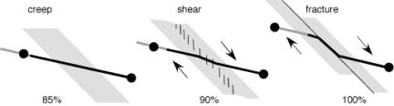
Fig.8. An increase in
transducer sensitivity accompanies the progressive localization of shear in a
fault zone. For finite creep, a creepmeter at 30° to a fault measures creep
attenuated by 1/cos30. In
the case of a creepmeter rod dragged parallel to the fault the transducer
monitors the full slip of the fault.
An example as to the probable behavior of a creepmeter during an earthquake is afforded by the destruction of the Caltech creepmeter across the Superstition fault during the 1987 Superstition Hills earthquake. The pipe assembly of the Caltech creepmeter was destroyed by afterslip on the fault, but the stainless-steel wire length standard of this creepmeter was dragged through the fault zone intact. The creepmeter was not being recorded electronically at the time of the earthquake, and the limited range of the beam balance that held the wire in tension resulted in the wire detaching from the balance early in the afterslip process.
Slip on the fault during an earthquake tends to confine the normally broad shear zone of a creeping fault into a narrow shear zone. This enhances the sensitivity of the creepmeter to fault-parallel slip. (Figure 8). A creepmeter crossing a uniform shear zone at an oblique angle, ø, has a sensitivity to dextral slip such that the measured displacement must be multiplied by 1/cosø to derive true dextral slip. The narrowing of the fault zone during earthquake slip reduces this obliquity. In the extreme case, the rod would be bent to follow the fault zone, i.e. ø=0. The geometry of the bent rod would therefore need to be examined after the earthquake to determine the appropriate afterslip calibration factor. Carbon fiber rods are considerably tougher than the clays and soils of the fault zone. Hence, providing the remote end of the rod remains fixed securely to an engineered mount, the rod will be drawn through the fault zone despite large shearing forces in shallow soils.
Creepmeters, briefly installed in 1970 by Nason, used a continuous rotation potentiometer with a wire length-standard held in tension by a constant-tension spring motor, and this was able to maintain high-resolution over large range, limited only by the dynamic range of the strip chart recorders then available. Two minor problems attend this arrangement- a dead zone at the transition from track-maximum to track-minimum, and the tendency for the fiber to slip on the shaft.
Digital shaft encoders overcome the errors associated with continuous-turn potentiometers, however, the problem of shaft slip remains unless a beaded-cable or chain is used to connect the rotating shaft to the length standard. In the late 1980's Kerry Sieh devised a digital fault velocity meter for use in Parkfield based on a shaft encoder. During rupture this above ground slip meter records the time taken for equal increments of fault slip to occur. The arrangement requires limited data storage because no data are recorded only during the time that the fault is inactive.
 Fig. 9 Inexpensive slip meter with 3 m range
and 1 mm resolution. Power is
supplied by an ONSET data logger which records a sample at ten minute intervals
for a year (12 days at a 1 s sample interval in afterslip studies).
Fig. 9 Inexpensive slip meter with 3 m range
and 1 mm resolution. Power is
supplied by an ONSET data logger which records a sample at ten minute intervals
for a year (12 days at a 1 s sample interval in afterslip studies).
We have devised a simple rupture meter to capture coseismic slip and afterslip of up to 3 m. The instrument consists of a ten-turn precision potentiometer attached to a 30 cm circumference drum on which is wound 3 m of Teflon-coated stainless steel wire. The wire is attached to the drum and is wound in a single layer. The free end of the wire is attached to the creepmeter fault-crossing rod, and is held in tension by a constant-tension spring motor attached to the drum (Figure 9). A precision of 1 mm and an accuracy of 7 mm is obtained using an Onset H12 data logger. As in the low power system described above, the data logger switches power to the device for 10-15 ms before data are sampled. It then goes into a "sleep mode" between samples. A sampling interval of 10 minutes affords 12 months of self-powered operation from 4 AA cells. At one sample per second 12 days of operation can be stored before data must be downloaded.
We have also tested an extended–range LVDT sensor designed to measure pre-seismic, coseismic and post-seismic surface slip of more than 2 m to 10µm precision. The long range is achieved using a pair of coaxial LVDTs with through-going bores. A segmented multiple core is assembled from ferrite cores separated by non-magnetic spacers of identical length (Figure 10c). Linear displacement of the core assembly through the LVDT assembly ramps the measured voltage through the linear range of each transducer over a cumulative distance, limited only by the number of cores and spacers installed. For example, in our experimental prototype 20 cores separated by 19 spacers provide a total measurement range of 2.03 m. The ferrite-core string is supported in a transparent tube as shown schematically in Figure 10b.
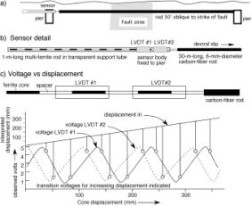
Figure 10a shows
a long range creepmeter across an active fault. 10b illustrates a string of ferrite-cores and spacers
arranged to be pulled through the LVDT by fault motion, and 10c illustrates the
voltage output from the two LVDTs.
LVDT#1 is shifted by approximately 1/2 a core length. A 3-channel data logger records the two
voltages and temperature. The data
are reconstructed from the linear portions of each LVDT output. Transition voltages for microprocessor
reconstruction of a 40 cm displacement signal are indicated in the figure by
circles. A displacement resolution of 6 µm is thereby obtained over a
measurement range of >2 m. The two LVDT's each consume 6 mA at 8V.
Measurements with segmented cores reveal that each LVDT has two usable measurement states: the first corresponds to the linear range when the central core links the primary coil to the two surrounding secondary coils, the second, with opposite polarity and reduced linear range, when a spacer lies at the center and the two cores adjoin the secondary coils. The output from this arrangement is an approximate triangular wave. To avoid using the non-linear region near the crest of each wave, the offset between the two transducers is shifted so that the linear range from one corresponds to the turning point of the other. The use of two LVDT's in close proximity requires the use of a shared oscillator to prevent mode-pulling.
At a sample rate of 1Hz, the multiple LVDT sensor can record cumulative slip accurately for fault-slip velocities less than 0.01 m/s. LVDT's are bandwidth limited to approximately 200 Hz and at this sampling rate fault slip velocities of up to 2 m/s could be captured. A sensor suited to recording the rapid velocities anticipated in surface ruptures associated with a ripple-type pulse (Andrews and Ben Zion, 1997) would therefore need to adopt different technology. A shaft encoder with a digital counter would provide a simple method to measure slip velocities of several 3 km/s.
future Creep investigations
Creepmeters are absent in the
planned inventory in the Plate Boundary Observatory instrumental pool, partly
because a large array of creepmeters has already been installed and operated by
the USGS for the past 30 years, and partly because creep is usually considered
a surface phenomena contributing little to our understanding of the process
zone of earthquakes. However, the
creepmeter pool is based on old technology. In particular, the absence of stable piers in the California
creep array is likely to hinder the interpretation of strain and displacement
data from the planned expansion of continuous GPS tracking sites and borehole
strainmeters.
Surface creep occurs in northern
California on the Maacama, Concord, Hayward, and Green Valley faults, on the San Andreas fault in central
California, and on the Eureka Peak, San Andreas, Imperial, Superstition Hills
faults in southern California. The
reason why so many of California's faults creep remains speculative. Allen (1968) noted that an abundance of
low friction serpentenite in the fault zone might be the cause for surface
slip, and Sieh and Williams (1990) propose that thick water-saturated sediments
may be responsible for creep in the Coachella Valley.
Creep rates are demonstrably
modulated by strain-fields applied to the fault zone. These rate changes are most clearly expressed following the
stress changes imposed by nearby large earthquakes on creeping faults (Mavko et
al., 1985; Schulz et al., 1990; Galehouse and Lienkaemper, 2001, Simpson et
al., 2001; Lienkaemper and Galehouse 2002, Lyons and Sandwell, 2002). Surface creep accompanies slow
earthquakes at depth (Linde et al., 1992). Some observational data suggest that creep rate
changes precede local earthquakes (Sylvester, 2004) as may be expected from
theoretical considerations. For example, post 1997 slowing in the creep rate on
the Hayward fault at Fremont to 5.1 mm/year may signify stress changes related
to the future earthquake processes there (Figure 11).
Until now, the noise levels of
most creepmeters have prevented the full exploitation of the information
contained within creep signals.
Whereas considerable funds are typically expended in the installation of
GPS instruments whose anticipated maximum resolution is currently ≈1 mm, no
similar effort has been devoted to the monumentation of creepmeters whose
displacement resolution is ≈1 µm.
Strainmeter anchoring methods yield micron-level stability relative to
points at depth (Wyatt, 1982; Wyatt et al., 1982, Zumberge and Wyatt, 1998),
but there is no simple way to determine what constitutes an acceptable depth
for anchoring instruments close to fault zones. Very often a creepmeter monument is installed in
heterogeneous fault gauge and the symmetry of typical strainmeter anchors is
inappropriate due to the proximity of the fault (7.5 m from the monument in a
30-m-long, 30° oblique installation).
The Hayward creepmeter array provides a guide to an appropriate anchoring depth
in Bay Area muds. An inclinometer borehole at Fremont penetrates to ≈30 m below
the surface (Bilham and Whitehead, 1997; Bilham 1998) and the lateral
displacement noise level falls by a factor of 5 or so below 10 m depth (Figure
11). At shallower depths soils lag
or lead deeper fault motion by up to 5 mm, whereas the depth interval 10-20m
behaves monolithically to within 1 mm. However, in Fremont, an inferred splay
fracture from the main fault may be responsible for this abrupt decay in
surface noise-level below 10 m. The nearby helical pile monuments here are
anchored to 10 m depth.
Fig. 11. Creep on
the Hayward fault in the past decade has been monitored both by surface
creepmeters and by a borehole inclinometer that penetrates the fault between 20
and 22 m depth (due to the serendipitous 70°SW dip of the fault). The
2.5-m-long segment of the inclinometer hole crossing the fault tilts by
0.17°/year. Each vertical line represents the sequential measurement of 50 cm borehole segments
from the top to the bottom of the hole (dates indicated above) differenced from
a measurement in July1994. After initial borehole settlement (pre-July 1994
data are negative from zero), lateral noise falls off rapidly below 10 m
depth. The vector plot shows the
displacement of the top of the borehole ( in the hanging wall) relative to the
base (in the footwall).
The creepmeters described in this
article adopt relatively low level technological solutions to the measurement
of fault creep. They permit, in
principle, creepmeters with lengths of 10 m-100 m, although the longest yet installed is approximately 33
m. More complex measurements may
be envisaged that could surpass the accuracies available to mechanical
creepmeters. For example, fiber
optic methods are suitable where slip, and therefore strain is not excessive
(Zumberge and Wyatt, 1998), and provide a potential measure of interseismic
creep rates in boreholes drilled across fault zones at depth. Inclinometer holes similar to that
shown in Figure 11 equipped with continuous recording tiltmeters would permit
creep to be measured at depths of several km. Although the maximum creep signal
decays with depth, the noise level decays much faster. Therefore creep measurements at great depth may not necessarily be
advantageous. Automatic precision
levels monitoring horizontal bar-coded leveling staffs, could be adapted to
measure lateral slip across fault zones without the need for an oblique
fault-crossing length standard, although the disadvantage of surface
instruments is that they are prone to vandalism.
The promise of new data from PBO
describing the strain-fields applied to California's creeping faults suggests
that a corresponding improvement to the existing California creepmeter array
would be of great value. It is
likely that such an investment in instrumentation will result in a clearer
understanding of the physics of creep, an incremental improvement in the
utility of monitoring surface creep, and its increased adoption as a
fundamental tool for monitoring the earthquake cycle.
Acknowledgements
Creepmeter studies in California
are funded by the U.S Geological Survey NEHRP programs. This work has received generous support
from Malcolm Johnson, Doug Myren,
Vince Keller and Stan Silverman, and builds on the early contributions of Bob
Burfurd and Bob Nason. The maintenance of the Hayward creepmeters, undertaken
collaboratively with Kate Breckenridge and Scott Whitehead between 1993 and 1997, was resumed in 2004 by grant USGS 04
HQAG0008. Data may be viewed
unprocessed at http://quake.wr.usgs.gov/research/deformation/monitoring/data/sf.creep.7.html
and in processed form (with thanks
to Susanna Gross) at http://strike.colorado.edu/~sjg/creep
References
Allen, C. R., Luo Z., Qian H., Wen X., Zhou
H., and Huang W., Field study of a highly active fault zone: The Xianshuihe
fault of southwestern China, Geol. Soc. Am. Bull., 103, 1178-1199, 1991.
Allen, C. R., The tectonic environments of seismically active and inactive areas along the Andreas fault system. In Conference on geologic problems of the San Andreas Fault system, Stanford California 1967. Stanford University Publications, Geological Sciences. 11, 70-80, 1968.
Allen, C. R., Wyss, M., Brune, J. N.,
Grantz, A., and Wallace, R. E., 1972, Displacements on the Imperial,
Superstition Hills, and San Andreas faults triggered by the Borrego Mountain
earthquake: U. S. Geological Survey Professional Paper 787, p. 87-104.
Andrews, D. J. & Ben-Zion, Y., 1997.
Wrinkle-like slip pulse on a fault between different materials, J. Geophys.
Res., 102, 553.
Behr. J., Bilham R and P. Bodin, Eureka Peak
Afterslip following the June 28, 1992 Landers Earthquake. Bull. Seism. Soc.
Amer., 84(3), 826-834, 1994.
Bilham, R. Measurements of Surface Stability of Engineered Geodetic Control Points, in The Global Positioning System for the Earth Sciences, 202-210, Nat. acad. Press Washington D.C. 1997 pp. 239.
Bilham, R., and J. Behr, A two-depth model
for aseismic slip on the Superstition Hills fault, California, Bull. Seism.
Soc. Amer., 82, 1223-1235, 1992.
Bilham, R., and S. Whitehead. Subsurface
Creep on the Hayward Fault, Fremont California, Geophys. Res. Lett. 24, 1307-1310.
1997.
Bilham, R., Borehole Inclinometer Monument for Millimeter Horizontal
Geodetic Control Accuracy, Geophys. Res. Lett. 20, 2159-2162, 1993.
Bilham, R., Sinestral creep on the Xianshuihe
Fault at Xialatuo in the 17 years following the 1973 Luhuo earthquake, Proc.
PRC-US Bilateral Symposium on the Xianshuihe Fault Zone, October 1990, Chengdu,
China. Seismological Press, Beijing, 226-231, 1992.
Bilham, R., Surface slip subsequent to the 24
November 1987 Superstition Hills, earthquake, California, monitored by digital
creepmeters, Bull. Seism. Soc. Amer.,
79(2), 425-450, 1989.
Bodin. P., R. Bilham, J. Behr, J. Gomberg,
and K Hudnut, Slip Triggered on Southern California Faults by the Landers,
Earthquake Sequence. Bull. Seism. Soc. Amer. 84(3), 806-816, 1994.
Bürgmann, Roland, Schmidt, D., Nadeau, R. M., d'Alessio,
M., Fielding, E., Manaker, D., McEvilly, T. V. , Murray, M. H., 2000,
Earthquake Potential along the Northern Hayward Fault, California: Science, p.
1178-1182.
Dogan, A. H. Kondo, O Emre, Y. Awata s. Ozalp, Triggered
slip on the Ismet pasa segement of the 1944 Bolu-Gered surface rupture by the
1999 Izmit earthquake, North Antolian Fault, Turkey. European Geophysical Society, Geophysical research Abst. 15,
11520, 2003.
Galehouse, J. S. and J. J. Lienkaemper, Inferences drawn
from two decades of Alinement Array measurementsof creep on faults of the San
Francisco Bay region, Bull. Seism. Soc. Amer., 93, 24152433, 2000.
Gomberg, J., P. A. Reasenberg, P. Bodin, and R. A. Harris,
2001, Earthquake triggering by transient seismic waves following the Landers
and Hector Mine, California earthquakes. Nature 411, 462-466.
Johnson, H. and D. Agnew, "Monument
motion and measurements of crustal velocities," Geophys. Res. Lett., vol.
22, pp. 2905-2908, 1995.
Kilb, D, J. Gomberg, and P. Bodin, 2000,
Triggering of earthquake aftershocks by dynamic stresses, Nature, 408, 570-574.
King, G.C.P., R.G. Bilham, J.W. Campbell, D.P. McKenzie and M. Niazi,
Elastic strain fields due to fault creep events observed by invar wire
strainmeters in Iran, Nature (Lond), 253, 1975.
Lee, J.C., Jeng, F.S., Chu, H.T., Angelier,
J. and Hu, J.C., 2000. A rod-type creepmeter for measurement of
displacement in active fault zone: Earth, Planets, and Space, 52, 5, 321-328
Lienkaemper, J. J., Galehouse, J. S., and R.
W. Simpson, Long-term monitoring of creep rate along the Hayward fault and
evidence for a lasting creep response to 1989 Loma Prieta earthquake, Geophys.
Res. Lett., 28, 2265-2268, 2001.
Linde, A. T., M. T. Gladwin, M. J. S.
Johnston, R. L. Gwyther, and R. Bilham, 1996. A Slow Earthquake near San Juan
Bautista, California, in December, 1992, Nature., v383, 65-68.
Lyons S., and D. T. Sandwell, Fault Creep Along the
Southern San Andreas from InSAR, Permanent Scatterers, and Stacking, J.
Geophys. Res.,
108(B1),
2047, doi:10.1029/ 2002JB001831, 2003.
Mavko, G., S. Schulz, and B. Brown, 1985,
Effects of the 1983 Coalinga, California, earthquake on creep along the San
Andreas fault, Bull. Seis. Soc. Am.,
75, (2), 475-489.
Nason, R.D., F. R. Philippsborn, and P.A
Yamashita, Catalog of creepmeter measurements in central California from 1968
to 1972, U.S.G.S. Open File Report 74-31.
Savage, J.C., and M. Lisowski, Inferred depth
of creep on the Hayward fault, central California, J. Geophys. Res., 98,
787-795, 1993.
Schultz, S. S. Catalog of creepmeter
measurements in California from 1966 through 1988. U.S.G.S. Open File Report 89-650.
Schulz, S., Mavko, G., and Brown, B., 1990,
Response of creepmeters on the San Andreas fault to the earthquake, in:
The Coalinga, California, Earthquake of May 2, 1983, Rymer, M.J. and Ellsworth,
W.L., eds., U.S. Geological Survey Professional Paper, P1487, 409-417.
Sieh, K., and P. Williams, 1990, Behavior of
the southernmost San Andreas Fault during the past 300 years, J. Geophys. Res. 95, 6629-6645.
Simpson, R. W.,
Lienkaemper, J. J., and J. S. Galehouse, Variations in creep rate along the
Hayward Fault, California, interpreted as changes in depth of creep, Geophys.
Res. Lett., 28,
2269-2272, 2001.
Sinvhal, H., P.N. Agarwal, G.C.P. King and
V.K.Gaur, (1973), Interpretation of Measured Movements at a Himalayan (Nahan)
Thrust, Geophys. J. R. Astr. Soc. 34(2) 203-210
Smith, S. W. and M. Wyss, Displacement on the
San Andreas fault subsequent to the 1966 parkfield earthquake, Bull Seism. Soc.
Am. 58, 1955-1973, 1968.
Sylvester, A, 2004.
http://www.geol.ucsb.edu/projects/geodesy/nail_lines/X0070_NYLAND_RANCH_NL.html
Wyatt, F., Displacement of surface monuments:
horizontal motion, J. Geophys. Res., vol. 87, pp. 979-989, 1982.
Wyatt, F., K. Beckstrom, and J. Berger,
"The optical anchor - a geophysical strainmeter," Bull. Seismol. Soc.
Am., vol. 72, pp. 1707-1715, 1982.
Yamashita, P. A. and R. O Burford (1973),
Catalog of preliminary results from an 18 station creepmeter network along the
San Andreas Fault system in central California for the time interval June 1969
to June 1973, U. S. Geol Survey Open File Rep[ort
Zumberge, M. A. and F. K. Wyatt, Optical
fiber interferometers for referencing surface benchmarks to depth, Pure Appl.
Geophys., vol. 152, pp. 221-246, 1998.