Fossil plants have long been used to infer paleoclimate and, by extension, paleoelevation. The most basic premise of paleobotanical theory is that plants that grow in warm climates look different from plants that grow in cold climates, and therefore if one or the other can be recognized in the fossil record we have a constraint on the climate in which the plants lived. In practice, paleobotany is fraught with more assumptions and inferences than most methods in the earth sciences, and the uncertainties associated with traditional paleobotanical analyses are huge. In many cases, though, paleobotany is the only method available for determining elevation history of a region.
Paleobotanical methods can be quite complex. Half of the analysis requires some identification or classification of the fossil flora; there are two main ways of doing this: 1) identification of the flora in terms of modern plants, or "nearest living relatives," and 2) characterization of the flora based on physiognomic characteristics. The second half of the analysis involves relating the fossil flora to some climate parameter or group of parameters, and further using these parameters to infer elevation. The climatic half of the analysis may involve estimates of mean annual temperature and growing season length, or less direct atmospheric parameters such as terrestrial lapse rate and mean annual enthalpy. In the following discussion, floral classification schemes are described first, followed by the methods of climatic and atmospheric analysis.
Fossil Classification
Nearest Living Relatives
The oldest and most common method for using paleobotanic data is to employ a scheme of "nearest living relatives" (NLR), also called the floristic method. In this method, the fossil flora are assigned a taxonomic classification that relates them to living flora; an assemblage of fossil flora is matched to the climatic conditions of an area containing a large number of NLRs (Wolfe, 1995). The use of NLR is widespread, despite having been shown both in theory and practice to be wholly unreliable. Not only do NLR analyses of the same flora often disagree widely in paleoclimate estimates, but the NLR method assumes that plants have not evolved in any significant way over the time period in question (Wolfe, 1995). When paleobotanists attempt to infer climates over millions or tens of millions of years, this assumption is obviously false. At best, then, the NLR method can be used only to identify very broad trends in climate.
The NLR method was used by MacGinitie (1953) in his original assessment of the Florissant fossils. He concluded that the Florissant flora represent a climate that was "warm temperate with relatively warm winters and hot summers," similar to the climates found today between latitudes of 20° and 30° in the northern Sierra Madre, northeastern Australia, or northwestern India. The elevation of the Florissant basin, MacGinitie (1953) argued, could have been no more than about 1 km.
Axelrod (1962, 1965, 1998) used a version of the NLR method in his assessment of fossil flora throughout the western United States. By relating fossil flora to "relict Tertiary forests," he identified a fossil flora from, for example, the Sierra Nevada as the ancestor of living forests in southeast Asia (Axelrod, 1965). His many studies of paleobotany throughout the western United States, all dependent on NLR methods, lend emphatic support to the Late Cenozoic uplift hypothesis.
Physiognomy
In an attempt to make paleobotanic analysis more quantitative, researchers began characterizing fossil flora on the basis of leaf characteristics, or physiognomy. By limiting the fossil samples to leaves only, the physiognomic method restricts the applicability but avoids the danger of using fossils, such as stems, seeds, or pollen, that are difficult to identify and may not display traits that are influenced by environmental factors.
Examples of fossil leaves from the Florissant flora, from MacGinitie (1953), showing various physiognomic characteristics used in the scheme of Wolfe (1993). Some of these characteristics include smooth versus toothed margins, varying width-to-length ratios, and blunt versus elongated leaf tips.
The phsyiognomic method begins by relating characteristics of modern leaves to climatic parameters (Wolfe, 1995). Leaf assemblages are collected from limited regions for which there is meteorological data available. The leaves are then measured for a variety of characteristics, including size, aspect ratio, shape, lack or presence of marginal teeth, and many others. From these measurements the percentage of samples within an assemblage displaying a certain trait are calculated. A multivariate correspondence analysis is applied to the percentages from all samples, giving the name CLAMP (Climate-Leaf Analysis Multivariate Program) to the method. Wolfe (1994) found that, in modern assemblages, 70% of the physiognomic variation could be explained by temperature and water stress. Application of the CLAMP method to fossil flora assumes that if climatic parameters can explain physiognomic variation, then that variation can be used to predict climatic parameters.
Example of a plot generated by physignomic leaf analysis (Forest et al., 1999). Click on the image for a larger view and explanatory caption.
The CLAMP method requires that an assemblage contain upwards of 20 species, each of which needs to be scored for roughly 30 physiognomic properties. But CLAMP provides a statistically sound, objective method for characterizing an assemblage of woody dicotyledons. Because the method is purely mathematical—leaves are measured, assemblages are treated with a correspondence analysis, etc.—there is little room for the subjectivity that taints the NLR method.
Indeed, the most important shortcoming of the CLAMP method is well-hidden behind the statistical rigor. The problem is that CLAMP is a purely statistical method; there is no quantitative physical or biological theory behind the classification of assemblages or the correspondence analysis. For example, although a characteristic such as leaf size may be found to predict mean annual temperature quite well, no botanical study has yet provided a thorough physiological or physical explanation as to why leaf size is related to temperature. Also, the scoring of 30 or more physiognomic states assumes that these characteristics are independent, an unlikely assumption for evolving flora. Qualitative explanations for the characteristics abound, many of which are quite reasonable and suggest that the physiognomic method is on the right track. The theoretical questions still remain, though, and in the CLAMP method there is always the uncertainty that perhaps toothed leaves (or large leaves, narrow leaves, elongated leaves, etc.) in the Tertiary were not responding to the same environmental stress as toothed leaves today.
Climate and Elevation analysis
With the exception of MacGinitie (1953), all researchers who have studied the Eocene Florissant flora and other relevant flora in Colorado have attempted to quantitatively estimate the paleoclimate in terms of some representative environmental parameters. Below, the most commonly used of these parameters are defined and explained.
Mean Annual Temperature
Mean annual temperature (MAT) is thought to be a general indicator of climate, shows strong correlation to plant physiognomy when analyzed with the CLAMP method, and can often be estimated to within 1° C (Forest et al., 1995). However, MAT by itself contains no information about elevation; it must be used in conjunction with other variables. A variation of MAT is the mean annual range of temperature (MART), the difference between cold and warm months. The combination of MAT and MART was used by Axelrod (1998) to place fossil plants from throughout the western United States, including the Florissant fossils and other Rocky Mountain Eocene floras, at elevations significantly lower than today.
Example of paleobotanic elevation analysis from MAT and MART (Axelrod, 1998). Click on image for larger view and caption.
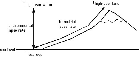
Lapse Rate
Lapse rate is the rate of temperature change with altitude, measured in °C / km. The environmental lapse rate is the change in temperature in a vertical column of air, whereas the terrestrial lapse rate is the change in temperature along the land’s surface (Meyer, 1992).
Schematic showing the difference between environmental and terrestrial lapse rates. Because of daytime heating of near-surface air along the topographic slopes, Thigh-over land is often much higher than Thigh -over water, even when measured at the same elevation (Meyer, 1992). Thus, the terrestrial lapse rate is lower than the environmental lapse rate.
It is the terrestrial lapse rate that is of interest in paleobotanical studies. In modern settings, the lapse rate is calculated from altitudes and long-term records of mean temperature. The lapse rate is related to the mean temperatures and elevation by the equation:
elevation = (T(high) – T(low)) / terrestrial lapse rate
Lapse rates generally vary from 3-9° C/km for regions with significant topography (Forest et al., 1999). The above equation would work wonderfully if it weren’t for a few simple problems: Terrestrial lapse rate is highly variable and poorly understood, even in modern climates, and inferring paleo-lapse rates is often nothing more than educated guesswork.
Moist static energy
In an attempt to avoid the uncertainties in calculations based on lapse rate, Forest et al. (1995) sought an atmospheric parameter that could be related to altitude by physical theory rather than relying upon empirical observations. What they came up with is a thermodynamic quantity called moist static energy. The moist static energy, h, is defined as the total specific energy content of air, excluding the kinetic energy. Thus, it is essentially the sum of the enthalpy, H, and the gravitational potential energy:
h = H + gZ
where g is gravitational acceleration and Z is altitude. Moist static energy is a suitable parameter for paleoelevation studies because it is mostly conserved as a parcel of air travels upward in the atmosphere, and because the flow of the upper troposphere makes moist static energy nearly invariant with longitude. Because moist static energy h in the above equation is the same at sea level and at altitude, if the enthalpy H is known both at sea level site and a corresponding upland site, the elevation of the upland can be calculated:
Z = H(sea level) – H(high) / g
First, schematic diagram of the conservation of mist static energy with elevation (Forest et al., XXXX). Second, zonal distribution of mean annual moist static energy in modern North America. Click on images for a large view and descriptive caption.
Thus it becomes necessary to estimate the mean annual moist enthalpy of two areas, one at sea level and the other at some unknown elevation. This is where the CLAMP floral method is useful. Mean annual enthalpy can be related to leaf characteristics by the multivariate correspondence analysis described above. Two fossil flora samples from the same latitude are required and, more importantly, it must be assumed that the moist static energy in the region spanned by the flora is invariant with longitude (Forest et al., 1995). The validity of the zonal invariance assumption is a matter of debate, as the zonal distribution of moist static energy seems to be perturbed by both continentality and topography; the former is difficult to infer for past climates and the latter is, of course, one of the unknowns motivating the research in the first place. The uncertainties derived from the enthalpy determination and the assumption of zonal invariance add up to a total elevation error of about 1 km.
Summary of Colorado studies
In south-central Colorado, the different methods of estimating paleoelevations have yielded vastly different results, fueling the debate over possible Late Cenozoic uplift of the western United States. As discussed previously, MacGinitie (1953) using the qualitative NLR method to classify the Florissant fossils as belonging to a warm, mild climate at a low elevation. Epis and Chapin (1975) adopted the conclusion of MacGinitie (1953) and interpreted the low-relief Late Eocene erosion surface of south-central Colorado in terms of this low-elevation constraint. MacGinitie’s (1953) estimated elevation was 300-900 m, requiring at least 1.6 km of uplift since the Late Eocene to bring Florissant to its current elevation of 2.5 km.
Gregory and Chase (1992) applied a physiognomic multivariate correspondence method to determine the MAT of the Florissant flora and the lapse rate calculation of Meyer (1986, 1992) to find the paleoelevation. Because Meyer’s lapse rate calculation requires an estimation of sea level, Gregory and Chase (1992) performed two calculations. In the first, the sea level temperature was projected inland by taking into account the effects of continentality, base level, and latitude; in the second calculation, the sea level temperature was inferred directly from coastal data. Both calculations yielded a result very similar to the present elevation of Florissant: 2.3 ± 0.4 km and 3.2 ± 0.8 km, which overlap between 2.4 and 2.7 km. Using the same method, this estimate was later revised upward to 3.1 km, about half a kilometer higher than the present altitude (Gregory and McIntosh, 1996).
Wolfe et al. (1998) used the CLAMP approach to relate the Florissant flora—and many other flora—to various environmental parameters, and then calculated the paleoelevation from moist static enthalpy. This method requires no assumption of lapse rate and yielded a result of about 3.5 km, similar to the revised estimate of Gregory and McIntosh (1996) and roughly 1 km higher than the present elevation.
Wolfe et al. (1998) and Gregory and McIntosh (1996) also analyzed Oligocene assemblages from the Creede flora of the San Juan mountains and the Pitch-Pinnacle of the Sawatch Range. The flora from the Creede caldera, analyzed by the CLAMP method and estimates of terrestrial lapse rates from Oligocene, yields a paleoelevation of ~3.9 km for the Creede lake deposits (Wolfe et al., 1998). The analysis of the Pitch-Pinnacle flora is more complicated, however, because it’s age of 32.9-29 Ma straddles the time of the dramatic global Early Oligocene temperature drop, as recorded by marine stable isotopes and terrestrial plants (Gregory and McIntosh, 1996). Comparing the Pitch-Pinnacle flora to sea level assemblages and both pre- and post-temperature decrease yields paleoelevation estimates of 2-3 km or ~1 km.
Overall, recent quantitative analyses of fossil flora in Colorado indicate that in the Late Eocene and Early Oligocene, prior to the Oligocene temperature deterioration, elevations in the Colorado Rockies were at least as high as, if not higher than, modern elevations. This interpretation is a significant obstacle for the hypothesis of Late Cenozoic uplift. Eocene high elevations can be explained by Laramide uplift, but Late Cenozoic uplift would then require a decrease in elevation between the Eocene and roughly the Miocene, followed by another period of as-yet-unexplained uplift. Of course, data from only three fossil assemblages is not enough to determine an entire regions tectonic evolution, and so it is necessary to examine these paleobotanical results in the context of similar studies throughout the western United States. This is done in the Summary section that follows.