Magnetic Anomaly and Sea-floor Bathymetry Interpretation
Introduction
The use of magnetic anomalies as a way to understand past plate motions began in the 1950’s with ship tracks that measured the earth’s total magnetic field. The ability to interpret how and when the world’s ocean basins were formed was solidified by Vine (1966). Thereafter, the theory of ocean floor spreading was largely accepted. Today ocean floor anomalies are used as a way to interpret the relative past movement of tectonic plates.
Earth's Magnetic Field
The earth’s magnetic field is approximately the field of a magnetic, axially centered dipole. This dipole is described by most simply by the North Magnetic Pole, the South Magnetic Pole, and the Magnetic equator. At the magnetic equator, the magnetic lines of force are horizontal (Figure 1). Throughout time the earth’s magnetic field has undergone reversals. From the late Paleogene to the late Neogene (approximately 29-6 Ma for our interests) the earth has undergone 52 periods of normal polarity with matching periods of reversed polarity [Cande and Kent, 1995].

Figure 1. Earth’s Magnetic Field showing the directions both poles and either side of the magnetic equator. Bottom part of the figure shows elements of inclination and declination, except at the equator where only declination is shown [http://lrrpublic.cli.det.nsw.edu.au].
Formation of Magnetic Anomalies
It was originally thought that seafloor spreading invoked slow convection within the upper mantle, drift being initiated above an upwelling, and that continental fragments rode passively away from such a rift on a conveyor belt of upper-mantle material [Vine, 1966]. Today it is believed by most geoscientists that seafloor spreading is a passive process, whereby spreading occurs over a large diffuse area of mantle upwelling, instead, and that localized upwelling occurs as a result of and at spreading centers from the divergence of plates. As the material comes up to the earth’s surface, the magma is displaced orthogonal to the spreading center. Within the cooling lava are magnetic minerals that are susceptible to interaction with the earth’s magnetic field. Their susceptibility is termed coercivity. Because of this susceptibility, mineral domains of these magnetic grains align themselves with the earth’s magnetic field, and their magnetization is solidified as the rock rises through the Curie temperature. This magnetization causes the body to produce its own field, which also resembles a dipole. As stated previously, through time, the earth’s magnetic field reverses, which gives rise to rocks with normal magnetic orientations and rocks with reversed magnetic orientations. (Figure 2). These reversals give rise to the magnetic anomalies that we make use of today. The magnetic anomalies themselves are interpreted from data from both ship tracks and satellites (Figure 3). Theories have been proposed for the mechanisms controlling Earth’s magnetic field reversals, but the topic is still largely debated.
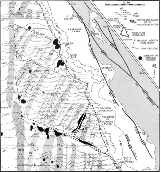
Figure 2. Interpreted magnetic anomalies in the Pacific Ocean off the coast of California. Positive anomalies are shaded grey as a convention. After Lonsdale (1991).

Figure 3. “Synthetic” magnetic anomaly profiles for the Juan De Fuca Ridge and the East Pacific Rise. The latitude of the profile is listed at the top of each profile. After Vine (1966).
Interpreting Magnetic Anomalies
Because the earth’s magnetic field is oriented differently at different latitiudes, as can be seen in Figure 1, the inclination of a compass needle will also vary with latitude. At the magnetic equator the value of inclination is zero. Because inclination component of magnetization of a N-S trending ridge does not contribute to the magnetic field outside the magnetized crust, the N-S oriented magnetization boundary at the magnetic equator creates no anomaly in the total field outside the magnetized body [Meng and Stock 2013]. What this means is that magnetic anomalies are very difficult to interpret at the magnetic equator, and easy to interpret at the poles where inclination is high.
Where magnetic anomalies can be interpreted, it may also be possible to date the magnetized rocks. This being the case, it is then possible to correlate magnetic anomalies across the earth’s ocean basins. In turn, these magnetic lineations form isochrons of the earth’s ocean basins, which are numbered relative to their age. As long as a spreading ridge is active, the direction of propagation should be orthogonal to the trend of the ridge. If a ridge is dead, the magnetic anomaly directly adjacent to the ridge records the time of last spreading. These elements turn out to be especially important in interpreting the capture of microplates along the western coast of North America.
Plates separated by a single spreading ridge should move in the same relative direction with more or less equal rates. If plate motions across a ridge change relative to the rest of the system, it can be assumed that this portion is now moving separately . This is the case with the many microplates seen along the western margin of North America. A good example is the Monterey mincroplate. Lonsdale 1991 notes (Figure 2) that the azimuth of the Morro transform fault is inconsistent with the almost east-west strike of the Shirley transform fault (assumed to record the direction of the Pacific-Cocos plate), and that the spreading center north of the Morro transform fault was moving at a slower rate than the Pacific-Cocos axes to the south. The observation that the spreading ridges are oblique to Pacific plate movement and had half spreading rates equal to half the estimated local speed of the Pacific plate suggests that at these latitudes the east-flank plate had stalled and become a new plate, the Monterey Microplate [Lonsdale 1991]. This is only true if the Pacific movement that Lonsdale is speaking to is relative to the North American plate. In order to resolve the movement of a specific plate, a reference system must be defined.
Use of Bathymetry
The use of bathymetry in tandem with magnetic anomalies is key to their interpretation, as is noted in Klitgord and Mammerickx (1982). In their paper they note that besides delineating major fracture zone trends and anomalous structural features, a bathymetric contour map indicates possible locations of minor fracture zones that might affect the magnetic anomaly pattern, and that the present crest of the East Pacific Rise is delineated in the bathymetry as regional basement high, whereas spreading centers that were abandoned during plate reorganizations are seen as combination of regional swells and narrow median troughs. Thus, it is possible to identify fossil spreading centers from the bathymetric data (Figure 4).
Abyssal Hills also play an important role in the interpretation of magnetic anomalies. Because magnetic anomaly data is not easily interpreted everywhere, it helps if there is another feature of the seafloor that parallels their trend. This is the case with Abyssal Hills [Menard and Mammerickx, 1967]. Because abyssal hills run parallel to the magnetic lineations, it possible to use them to steer magnetic interpretations where it might not otherwise be possible [Lonsdale, 1991].
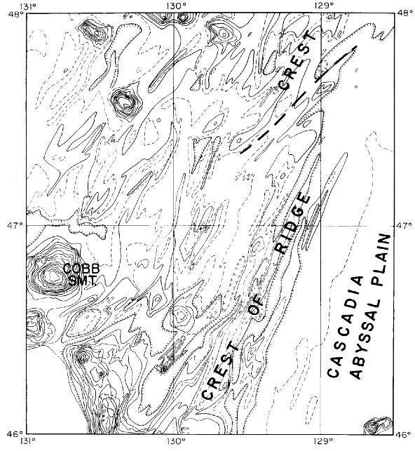
Figure 4. Topographic profile of part of the Juan De Fuca spreading ridge dashed marks are linear offsets. After Menard and Memmerickx (1967).