|
Turbulence Sensor
Turbulence Measurements
TLS Package

|
TLS Turbulence Package:
Turbulence Measurements
The advantage of the TLS turbulence data is that no assumption of significant importance on the result, such as the choice of the size of the averaging window when using the Reynold’s averaging technique, is made. The only assumptions are:
- the turbulence is locally isotropic, which is a good assumption for high Reynolds’number flows, and
- Taylor frozen hypothesis is valid (
 ), which accuracy is very good over short time intervals. ), which accuracy is very good over short time intervals.
Under these assumptions, the TLS provides unique high-resolution measurements of inertial range turbulence which can be computed with great accuracy as often as every 0.25 sec. In the TLS profiling mode of operation, using 1 second spectra to estimate inertial-range turbulence statistics is equivalent to spatially averaging regions of 0.5 m in the vertical (for an ascent/descent rate of 0.5 m/s) and U m in the horizontal where U is the streamwise horizontal wind velocity. This therefore corresponds to two-dimensional (x,z) regions of 0.5*U m2 and in the constant altitude mode of operation, the spatial averaging corresponding to 1-second spectra is U m.
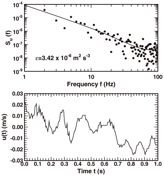
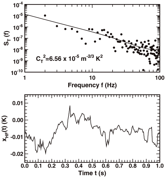
The inertial-range turbulence statistics (CT2 and ε) are computed by fitting the high-resolution temperature and velocity spectra to theoretical curves that model both a noise floor and the characteristic -5/3 power law of inertial-range turbulence (i.e., the spectral power is proportional to f 5/3 in the inertial range).
To satisfy the Taylor ’s frozen hypothesis, estimates are typically made from 1-second spectra which, thanks to the high-sampling rate and fast-responses of the CW and HW probes, contain enough data points in the inertial range to achieve good accuracies. With 1-second spectra and temperature/velocity data sampled at 200 Hz (sampling frequency of the first version turbulence packages), N=50 Fourier coefficients out of the 100 available are typically used for the fit, thus providing an accuracy better than 15%.
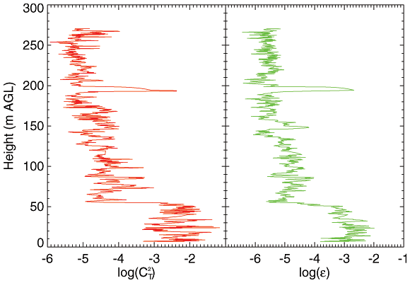
Below are examples of turbulence profiles (CT2 and ε) that the TLS typically provides. These profiles depict the vertical turbulent structure of the nocturnal boundary layer (NBL) and of the residual layer above it. The vertical resolution is about 0.5 m.

Click on image for larger version.
These high resolution profiles capture the sharp drop of turbulence around 50 m AGL that characterizes the top of the NBL, while in the residual layer (~195m AGL), a thin layer of strong turbulence intensity, which origin is yet to be determined, has been detected. |
|