A Closer Look at Salt Tectonics
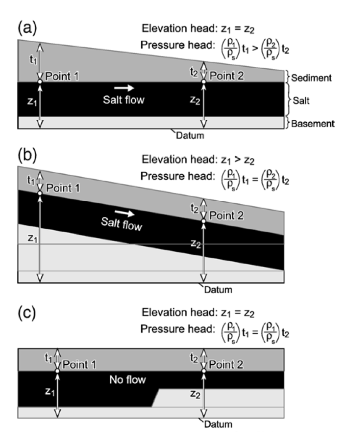
Before we can understand various salt structures, we must understand what drives salt tectonics. The most important factor to recognize is that salt flow does not actively drive salt tectonics, but salt passively reacts to external forces (Jackson & Talbot, 1986). It used to be widely accepted that salt tectonics was driven by salt buoyancy, where both the salt and overburden were treated as fluids with different densities. Once it was widely recognized that overburden strength was an important control on salt tectonics, differential loading was determined the controlling factor of salt flow. Salt buoyancy remains important for the continuation of diapir growth, but not the initiation (Jackson and Talbot, 1986). There are three main types of loading that drive salt flow: gravitational, displacement and thermal loading (Hudec & Jackson, 2007). This article will focus on gravitational loading because that is the driving force behind salt tectonics in the Western U.S. Gravitational loading is controlled by gravitational forces within the evaporite layer and the weight of the overburden. It can be explained using the concept of hydraulic head, where fluids flow from high head to low head, and in instances where head is constant, the salt remains stationary (Fig 8., Hudec and Jackson, 2007). There are two main factors that resist salt flow: the strength of the overburden and the boundary drag on the top and base of the salt layer. Salt will flow only if forces driving salt flow are greater than forces resisting it.
Once salt begins to flow, there are three main stages of structural development: reactive, active and passive diapirism (Fig. 9, Vendeville & Jackson, 1992). Reactive diapirism is vertical salt flow that reacts to differential unloading. Once differential unloading stops, reactive diapirism will stop. Diapirism will only continue if there is a density contrast between the salt and overburden and the salt is buoyant enough to continue flowing. This process is called active diapirism. Once the salt breaks through the surface, passive diapirism begins. This is continued growth of the surfaced diapir due to continual sedimentation (Vendeville and Jackson, 1992).

Paradox Basin
This page will focus on two main salt features in Paradox Basin: (1)Valleys developed by collapsed salt walls and (2) the Needles District, an extensional fault array due to incision of the Colorado River. The Paradox Basin (Fig. 10) was originally interpreted as a pull-apart basin of Pennsylvanian age (Stevenson & Baars, 1987), but it was later established that the evaporite basin is a result of plate flexure from the Ancestral Rockies uplift (Barbeau, 2003). Specifically, the shape, subsidence history, stratigraphic architecture, and structural observations all provide evidence of the flexural style of the Paradox Basin from loading of the Uncompahgre uplift. Figure 11 demonstrates how a flexural basin model fits quite well to the Paradox Basin profile that was determined by well data.

Salt Walls
The salt walls in the northeastern Paradox Basin (Fig. 12) are the result of diapiric growth as sediment was shed from the Uncompahgre uplift onto the evaporite sequence. Sediment deposition on top of the Paradox Formation caused differential unloading and salt to flow to the southwest. The presence of flexural normal faults below the evaporite sequence were linear features that perturbed lateral salt flow and caused salt to flow upwards, forming salt walls. Figure 13 is a structural reconstruction of salt wall development from the Pennsylvanian to the Late Jurassic. Note how the thickness of the sediments change due to growth of the salt wall and how salt wall growth stops once salt welds develop in the Permian, denoted by two black dots. These reconstructions were done using information from geologic mapping, seismic reflection, and well logging.
 Figure 12. Map of the Paradox Basin showing location of salt walls. Figure from Trudgill, 2011.
 Figure 13. Structural restoration along A-A' in figure 12 from the Pennsylvanian to Jurassic. Figure from Trudgill, 2011.
These salt wall have subsequently collapsed, creating wide valleys that are cross cut by rivers (Fig. 14). This is where the Paradox formation and Paradox Valley get their names because it seemed paradoxical that valley would develop perpendicular to rivers. Dissolution of the evaporite layer due to groundwater interaction caused subsequent collapse of the overlying sedimentary sequences (Fig. 15, Gutierrez, 2004). It has also been argued that these valleys are the result of regional extension and that salt dissolution plays a minor role (e.g. Ge and Jackson, 1994). Gutierrez, 2004 uses the presence of the thick cap rock above salt walls, subsidence deformation structures, structures inconsistent with regional extension, evidence of recent dissolution structures and aseismicity as evidence for dissolution driven subsidence creating the observed valleys.
 Figure 14. Topography of collapsed salt walls in western Colorado showing cross cutting rivers. Figure from Gutierrez, 2004.
 Figure 15. Types of structures that can develop due to dissolution driven subsidence. Figure from Gutierrez, 2004.
The Needles District
The Needles District, Canyonlands, Utah is an active array of extensional faulting due to unloading from the Colorado River (Fig. 16). Incision of the Colorado River drove flow of gently dipping salt from the southeast to the northwest, toward the canyon. This lateral salt flow instigated deformation and brittle failure of the overburden (Baker, 1933; (Mcgill & Stromquist, 1979; Moore & Schultz, 1999). Numerical modeling of the Needles District has shown that faulting propagated from the river to the southwest and younger grabens are more mature and symmetrical (Walsh & Schultz-Ela, 2003). Models have also demonstrated the importance of preexisting weaknesses in fault propagation and geometrical development in that the spacing of weak zones affect graben style and interaction (Fig. 17, Allken et al., 2013). The implementation of Interferometric Synthetic Aperture Radar (InSAR) shows subsidence rates of ~2 mm/yr and similar rates of uplift within the Colorado River adjacent to the Needles that stops downstream (Fig. 18, Furuya et al, 2007).
 Figure 16. Fault map of the Needles District from Schutz-Ela and Walsh, 2002.
 Figure 17. Block models i, ii, and iii show graben interaction in the Needles District. Models a, b, and c are numerical models that compare well with the ones above. Models a and b have a salt thickness of 50 m and preexististing weaknesses offset 600 and 1000 m, respectively. In model c, preexisting weakness offset is 1000 m and salt thickness is 100 m. Figure from Allken et al., 2012.
 Figure 18. InSAR results from ERS scenes ranging from 1992-2001. Red shows movement away from the satellite and blue shows movement toward the satellite. Figure from Furuya et al., 2007.