|
 |
| Chu Home | People | Projects | Publications | Classes | Contact | News & Events |
McMurdo Project Detail: |
McMurdo Project: Results from Prior CampaignsHighlighted below are the main scientific results obtained from the prior campaigns made with the Fe Boltzmann lidar. More details can be found in Publications. Thermal Structure from Ground to 110 km at High Southern Latitude
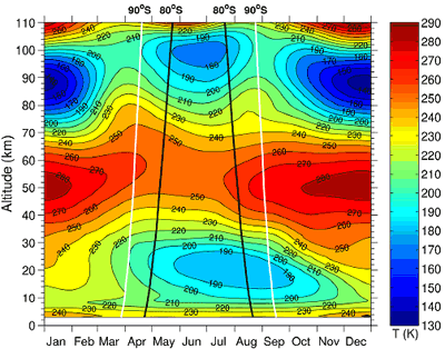
Figure 1. South Pole temperature climatology obtained by combination of Fe temperature, Rayleigh temperature, and GPS balloon sonde temperature [Pan and Gardner, JGR, 2003].
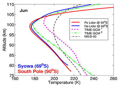
Figure 2. Comparison of the observed temperature at the South Pole and Syowa in June with the original TIME-GCM1 predictions, and the TIME-GCM2 predictions with weaker gravity wave forcing under June solstice conditions [Pan et al., GRL, 2002; Kawahara et al., JGR, 2002]. Polar Mesospheric Clouds and Heterogeneous Chemistry at 78°S
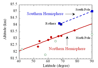
Figure 3. Mean PMC altitudes observed by lidars and triangulation measurements in both hemispheres. Errors are 0.05–0.16 km for filled circles and squares with extensive observations. The solid and dashed lines are linear fits to the northern and southern data. Open circles indicate limited datasets and are excluded in the fit [Chu et al., GRL, 2001; Chu et al, JGR, 2003, 2006].
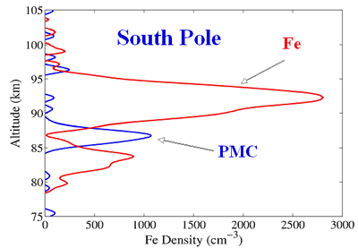
Figure 4. Simultaneous observations of the atomic Fe density and PMC backscatter signal at the South Pole by the Fe Boltzmann lidar operating at 372 and 374 nm, respectively. The signals are averaged between 3-6 UT on 19 January 2000. Complete depletion of Fe occurs at the PMC layer altitude [Plane et al., Science, 2004]. Mesospheric Fe Chemistry and Large-Scale Dynamics in Antarctica
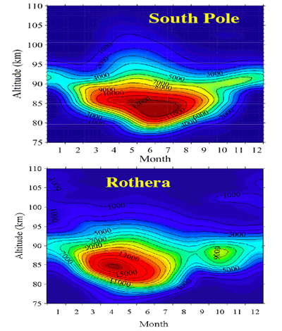
Figure 5. Seasonal variations of mesospheric Fe densities at the South Pole and Rothera [Gardner et al., JGR, 2005, 2011]
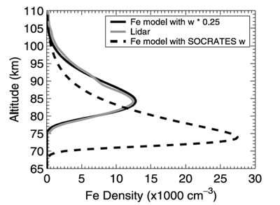
Figure 6. Comparison of the observed and modeled Fe layers in June at the South Pole. The predicted vertical wind, w, from the SOCRATES global circulation model is too large (w = -3.2 cm/s between 75 and 85 km), causing the layers to be displaced downward by about 10 km. Reduction of w by a factor of 0.25 produces good agreement with the observations [Gardner et al., JGR, 2005]. Gravity Wave Characterization and Wave Coupling in Antarctic Atmosphere
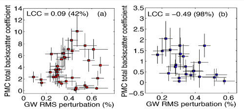
Fig. 7. PMC brightness (total backscatter coefficient) vs. GW strength (RMS relative density perturbation in the 30-45 km range) at the South Pole (a) and Rothera (b) [Chu et al., JASTP, 2009]. The linear correlation coefficient (LCC) is -49% with 98% confidence level at Rothera. Our lidar observations show statistically that Rothera PMC brightness is negatively correlated with the stratospheric GW strength but no significant correlation exists at the South Pole.
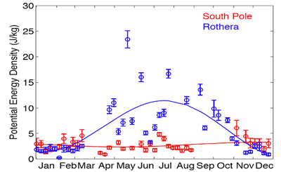
Figure 8. Seasonal variations of stratospheric gravity wave potential energy density in the 30-45 km at the South Pole and Rothera [Yamashita et al., JGR, 2009]. The data points represent weekly means while the solid lines are annual fits to the data points. Collaborative Studies on More Polar Aeronomy Topics
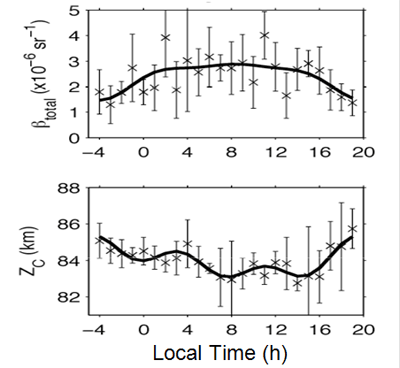
Figure 9. Observed diurnal, semi-diurnal, and terdiurnal variations of PMC brightness and centroid altitude at Rothera [Chu et al., JGR, 2003, 2006].
|