 G):
G):
T):
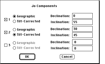
For instance, here we have designated a geographic direction that might be the modern dipole field at our locality as direction one, a second direction in tilt-corrected coordinates as direction 2, and we have not designated a direction 3. This will produce three panes in the J/J0 window: one for each of the two designated directions and a third called "Perp." which is the unit cross product of the two designated directions. Identifications of the directions is in the upper right part of the window. Because these are all vectors, both the J/J0 and derivative plots can be positive or negative. The base of the derivative rectangles indicates the zero in each pane. If only one direction is chosen, then the "Perp." direction is actually a scalar quantity representing the intensity in the plane perpendicular to the chosen direction.
What happens here is that we can represent any magnetization vector
 as a sum of three independent vectors:
 . Note that the three vectors need only
be independent (they must span 3-space) and do not have to be orthogonal. Thus
this technique will correctly separate an overprint from a characteristic
direction even if the two are much less than 90°ree; apart.
. Note that the three vectors need only
be independent (they must span 3-space) and do not have to be orthogonal. Thus
this technique will correctly separate an overprint from a characteristic
direction even if the two are much less than 90°ree; apart.
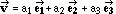
For example, the following sample's Zijderveld plot looks like:
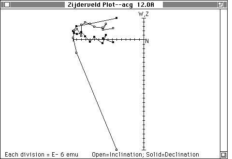
and produces a normal J/J0 plot looking like:
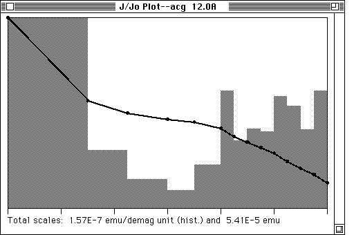
which reveals two components, here rather cleanly separated. If we estimate the two directions, say by doing least-squares fits (and possibly coming up with mean directions for the locality), we can make a component J/J0 plot that will look like this:
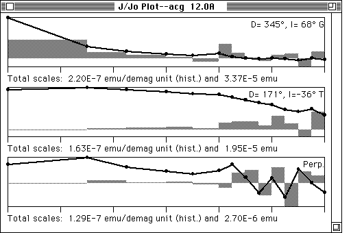
(the bottom ticks are at 100°ree; increments). This plot seems to substantiate the identification of the two components, but note the blip of the first component in the 400-425°ree; range; also note the erratic behavior of the orthogonal component, indicating an absence of a consistent magnetization along this axis.
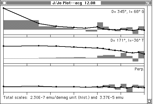
This tends to downplay spurious magnetizations, though weak characteristic directions might also become invisible.
 of
the mean (note
that N is usually so low for these sites that the rarely has great
significance beyond a guide to the scatter of the points). See the Samples, Sites, and Localities section below for more detail.
Grayed out if sites have
not been defined for this locality (see "Define
Sites..." in the File menu).
of
the mean (note
that N is usually so low for these sites that the rarely has great
significance beyond a guide to the scatter of the points). See the Samples, Sites, and Localities section below for more detail.
Grayed out if sites have
not been defined for this locality (see "Define
Sites..." in the File menu).
a
site can have and be displayed and a checkbox to permit the rejection of single
sample sites (which cannot have an estimated ). See the
Samples, Sites, and Localities section below.
 s; see the discussion in the .LSQ file format section). An arrow in the
declination and inclination/paleolatitude panes indicates the direction demagnetization is proceeding;
this arrow is absent when viewing by site or in the VGP latitude pane. When viewing by site, the
site mean of the extreme points is plotted, but arrows are not and squares are used to denote the use
of circle/plane fits. CAUTION: Note that the circle plotted is NOT at the position of the last point
used in the original fit, but at the projection onto the great circle of the point used that is farthest
from the starting end. In some circumstances (especially a plane fit not tied to the origin) this can
produce a misleading indication of the possible polarity of the sample.
s; see the discussion in the .LSQ file format section). An arrow in the
declination and inclination/paleolatitude panes indicates the direction demagnetization is proceeding;
this arrow is absent when viewing by site or in the VGP latitude pane. When viewing by site, the
site mean of the extreme points is plotted, but arrows are not and squares are used to denote the use
of circle/plane fits. CAUTION: Note that the circle plotted is NOT at the position of the last point
used in the original fit, but at the projection onto the great circle of the point used that is farthest
from the starting end. In some circumstances (especially a plane fit not tied to the origin) this can
produce a misleading indication of the possible polarity of the sample.