 |
 |
| Pielke Home | People | Publications | Images | Courses | News | Links | Contact |
| RESEARCH GROUPS @ CIRES > |
Image Gallery | |
Image |
|
Animations |
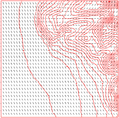
The case 15 Oct 2000 from the VTMX campaign was selected to test RAMS with initial and boundary conditions take from RUC20 forecast output. A three-nested grid system was defined as follows: the innermost grid 302 x 302 with 50 m grid spacing, the next grid 222 x 222 with 250 m grid spacing, and the outermost grid 125 x 125 with grid spacing of 1250 m. These grids are centered on Salt Lake City, Utah. In the vertical 31 levels were used with grid spacing of 50 m, near the surface, increase in depth to 188 m at 1.1 km. The terrain was taken from the 30 second data from USGS dataset. The animations A0400-4h-anim-10m.gif, A0400-4h-anim-50m.gif, and A0400-4h-anim-100m.gif correspond to the wind vectors over the innermost grid at 10, 50, and 100 m above the ground. The animations contain frames every 15 minutes for a total of 4 h of simulation. The terrain is depicted with red contours with contour interval of 50 m. The largest win vector magnitude is about 8 m/s. |
Images |
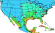
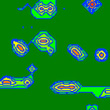
Large Eddy Simulation of the Lake-ICE case 19 January 1998 with RAMS; Adrian Marroquin* and Roger A. Pielke Sr.** NOAA Research-Forecast Systems Laboratory Boulder, Colorado *[In collaboration with the Cooperative Institute for Research in the Atmosphere (CIRA), Colorado State University, Fort Collins, Colorado] (**) Colorado State University, Fort Collins, Colorado, 80523-1375. Figure Captions Fig. 1: Sounding at Sheboygan, WI, for 1200 UTC 19 January 1998, taken from the Lake-ICE dataset available on the webpage. Winds barbs are in knots and the temperature and dewpoint are shown as solid curves. The other symbols correspond to the conventional skewT diagram. Fig 2: As for Fig. 1, except for 1500 UTC. Fig. 3: As for Fig. 1, except for 1630 UTC. Fig. 4: Lake-ICE RHI scan animation of lidar backscatter at an azimuth 104.5 for the time interval 16:35-17:31 UTC 19 January 1998. The lidar location is at the lower-left corner of the top rectangular figure. The horizontal axis spans 12 km and the vertical 500 m. Fig. 5: Horizontal cross section of temperature (K, 0.1 contour interval) at 1.5 km elevation from the LES output at the initial time, 1200 UTC 19 January 1998, for the outermost grid 54.45 km x 54.45 km (122 x 122). The terrain is shown in shades of color, with the colored bar indicating the elevations (m). The arrow indicates the location of the lidar. The land-water boundary is shown by the black north-south contour. Fig. 6: As for Fig. 5, except for wind (barbs, knots) at 1.5 km elevation. Fig. 7: Horizontal cross section of winds (barbs, knots) from LES output at the initial time, 1200 UTC 19 January 1998, and terrain (blue, contour interval of 2 m) for the innermost grid (10 km x 10 km, 202 x 202, 50 m grid spacing). The signs Snd-1, Snd-2, and lidar point to the location of model soundings shown in the next three figures. Fig. 8: Sounding at the Snd-1 location (see Fig. 7) from LES output at 1200 UTC 19 January 1998. The winds are shown by the red barbs (knots). The temperature (K), relative humidity%), and mixing ratio (g/Kg) are shown by the blue, black, and green curves. The scales for these variables are shown at the bottom of the figure while the scale elevation is shown on the right of the figure. The pressure (mb) levels are shown by the corresponding horizontal lines. Fig. 9: As for Fig. 8, except for Snd-2 location (see Fig. 7). Fig. 10: As for Fig. 8, except for the lidar location (see Fig. 7). Fig. 11: Horizontal cross section of winds (barbs, knots) at 100 m elevation and temperature (K, blue contours) at 2 m above the surface from LES output at 1530 UTC 19 January 1998, for the outermost grid (122 x 122, 450 m grid spacing). Fig. 12: Sounding at the lidar location from LES output for 1530 UTC 19 January 1998. Winds (knots) are shown by the wind barbs and the temperature (K) by the red curve. The dewpoint Temperature (k) is shown by the purple curve. The other symbols correspond to the convectional skewT diagram. Fig. 13: The animation shows the vertical velocity (m/s) from LES output interpolated to the lidar scan surface at 1.5 degrees for the innermost grid from 1530 to 1600 UTC 19 January 1998. The lidar is approximately at the center of the grid (see Fig. 7). Fig. 14: The animation shows the lidar backscatter PPI scan at 1.5 degrees elevation from 15:31-16:00 UTC 19 January 1998. This animation was copied from the Lake-ICE webpage. The lidar is located at the 0 mark on the left vertical axis. The scan coverage in the west-east direction is 10 km and from north to south is approximately 10 km. Fig. 15: The animation shows the evolution of the LES relative humidity (RH%, shades of color) in the boundary layer on a vertical cross section at an azimuth of 104.5 degrees for the innermost grid (horizontal axis with 202 grid points). The cross section passes over the lidar location at grid point 107. The animation spans from 1630 to 1730 UTC 19 January 1998. Shades into the dark red color indicate relative humidities above 80% while white shows RHs below 10%. Fig. 16: As for Fig. 15, except for the potential temperature (K). Light colors show temperatures below 272 K, while dark red show temperatures above 276 K. Fig. 17: As for Fig. 4, except for an azimuthal angle of 119.99 degrees and for a time interval 15:14-15:27 UTC. The horizontal axis spans from 2200 to 5500 m and the vertical 1 km. Fig. 18: Sounding from LES output (3 hours into the simulation) at the center of the domain valid at 1500 UTC 18 January 1998. The green and red curves represent the dewpoint temperature and temperature (K), respectively. Fig. 19: As for Fig. 4, except for an azimuthal angle of 148.50 degrees and for a time interval 12:25-13:49 UTC. The horizontal axis spans 10 km and the vertical 250 m. Fig. 20: Horizontal cross section (1 km above the surface) of model-generated vertical velocity (m/s) patterns with the modified initial/boundary fields at 3 h (valid at 1500 UTC). Fig. 21: Model sounding at 1800 UTC showing the modified temperature (K, red) and dewpoint (K. green) at the lateral boundaries. Fig. 22: Sheboygan WI sounding at 1800 UTC 19 January 1998 from Lake-ICE data. The right/left shows the temperature/dewpoint (K) and the winds are in knots. Fig. 23: As for Fig. 21, except for a sounding at the center of the innermost grid at the end of the 6th h (valid 1800 UTC 19 Janury 1998) into the simulation in which modified lateral boundaries for 1800 UTC were used. Fig. 24: As for Fig. 15, except for an RH animation that spans from 1630 to 1730 UTC. |
Video |
The movie file (8 Mb) is a perspective view of Hurricane Georges looking from the northwest. The horizontal plane shows the wind streamlines and surface pressure (color, in mb). The isosurface is total condensate. The animation begins at 0GMT on September 21, 1998. The model results are part of effort to examine the effects of topography on landfalling hurricanes and for another study on the effects of sea surface temperature on hurricane intensity. The RAMS model was integrated on a 5km mesh covering 230 East-West points and 105 North-South points. There were 27 points in the vertical extending to 26km above ground level. The model was integrated in a parallel mode, employing 64 processors at San Diego Supercomputer Center. Additional runs were completed on a cluster of 6 processors provided by project consultant, Joseph L. Eastman. The graphics were generated using the Environmental WorkBench (EWB) courtesy of SSESCO, INC. Please Note: The below video clip is in the .avi file format and requires that you have an AVI player installed and configured properly for your system. If you have difficulty when clicking on the below link, please visit the AVI Viewing Instructions page. |
Images |
Eastman, J.L., M.B. Coughenour, and R.A. Pielke, 2001: The effects of CO2 and landscape change using a coupled plant and meteorological model. Global Change Biology, In Press. (PDF) Figure 7: The seasonal domain-averaged contributions to maximum daily temperature due to f1-natural vegetation, f2-2xCO2 radiation, f3-2xCO2 biology, f12-interaction of natural vegetation and 2xCO2 radiation, f3-interaction of natural vegetation and 2xCO2 biology, f23-interaction of 2xCO2 for radiation and biology, f123-the interaction of all three factors. Figure 8: Same as Figure 7 except for minimum daily temperature contribution. Figure 9: Same as Figure 7 except for LAI (m^2 m-2). Figure 10: The number of significant differences for the KS test versus time of day for the factor contribution (indicated by the legend). The variables are defined in Table 7. |
Images |
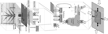
Pielke, R.A., 2001: Influence of the spatial distribution of vegetation and soils on the prediction of cumulus convective rainfall. Rev. Geophys., In Press. PDF)
Figure 10: Schematic representation of the simulated three-dimensional domains (from Avissar and Liu 1996).
Figure 12: Model output cloud and water vapor mixing ratio fields on the third nested grid (grid 4) at 21 GMT (Greenwich Mean Time) on 15 May 1991. The clouds are depicted by white surfaces with q_c = 0.01 g/kg, with the sun illuminating the clouds from the west. The vapor mixing ratio in the planetary boundary layer is depicted by the grey surface with q_v = 8 g/kg. The flat surface is the ground. Areas formed by the intersection of clouds or the vapor field with lateral boundaries are flat surfaces, and visible ground implies q_v < 8 g/kg. The vertical axis is height, and the backplanes are the north and east sides of the grid domain (from Pielke et al. 1997). Figure 16: Convective precipitation differences (current minus natural, contour by 0.5 mm/day) using a 9-point spatial filter for easier visibility. Light shading represents the 90% significance level for a 1-sided t-test. Dark shading represents the 95% significance level (from Chase et al. 2000). Figure 17: 200 hPa height difference (current minus natural landscapes). Contour interval is 20 m (from Chase et al. 2000). Figure 18: Difference in near-surface air temperature (current minus natural landscape) using a 9-point spatial filter for easier visibility. Contour intervals are 0.5, 1.0, 1.5, and 3.0 deg C. Light shading represents the 90% significance level for a 1-sided t-test. Dark shading represents the 95% significance level (from Chase et al. 2000). |
| Other Images |
Climate Prediction: An Initial Value Problem
|
Nondiscrimination Policy • Legal and Trademarks |